 Prodia
KalSea: Kalman Residual Forecasting with Spectrally Aligned Skipping for Training-Free Acceleration of Diffusion Transformers
SeaCache's gate decides when to skip the transformer. Small Kalman filters decide what to write on the skipped steps.
KalSea is a training-free cache for diffusion transformers. The spectrally aligned gate from SeaCache [1] decides when to run the full transformer. On skipped steps SeaCache reuses the last computed residual of the block stack; KalSea forecasts it with small Kalman filters that track a value and a damped trend. The gate, the threshold δ and the number of transformer evaluations (NFE) are the same for both.
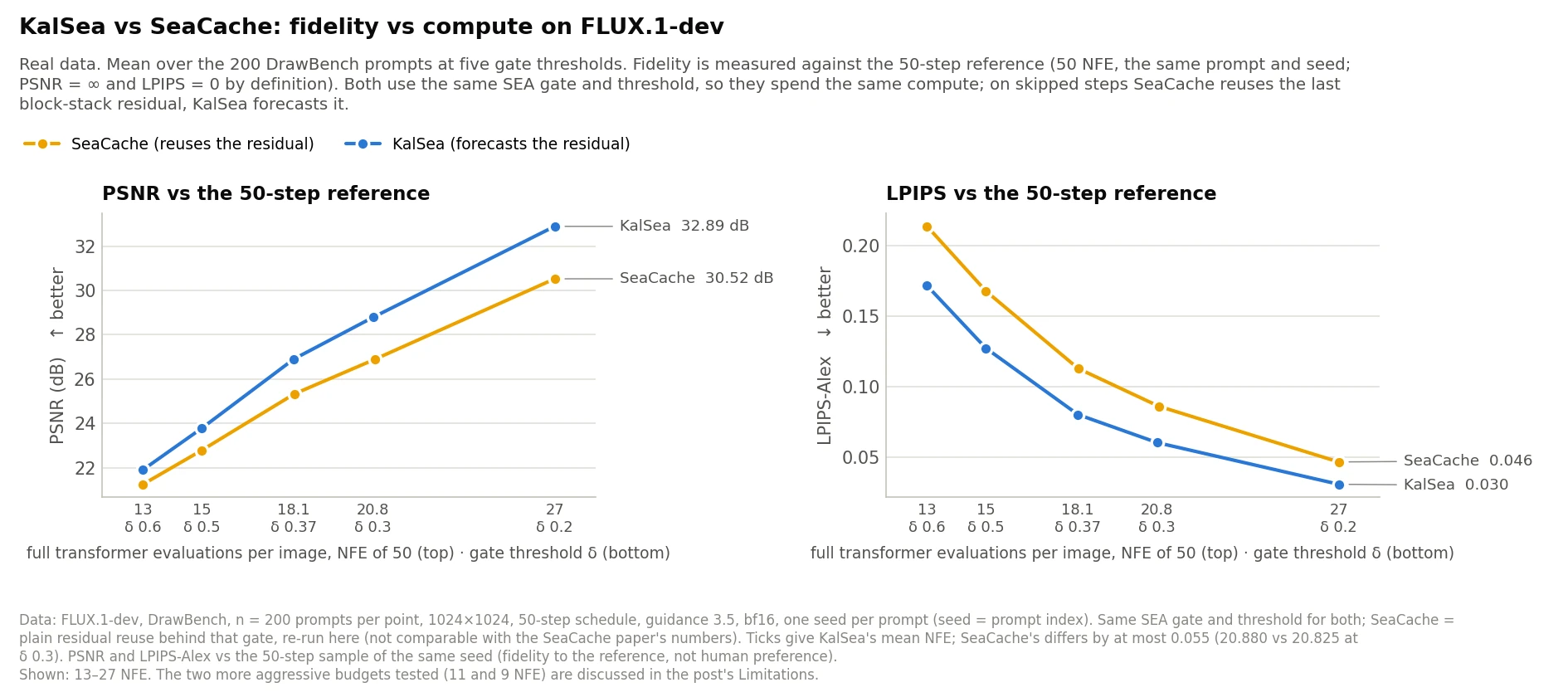
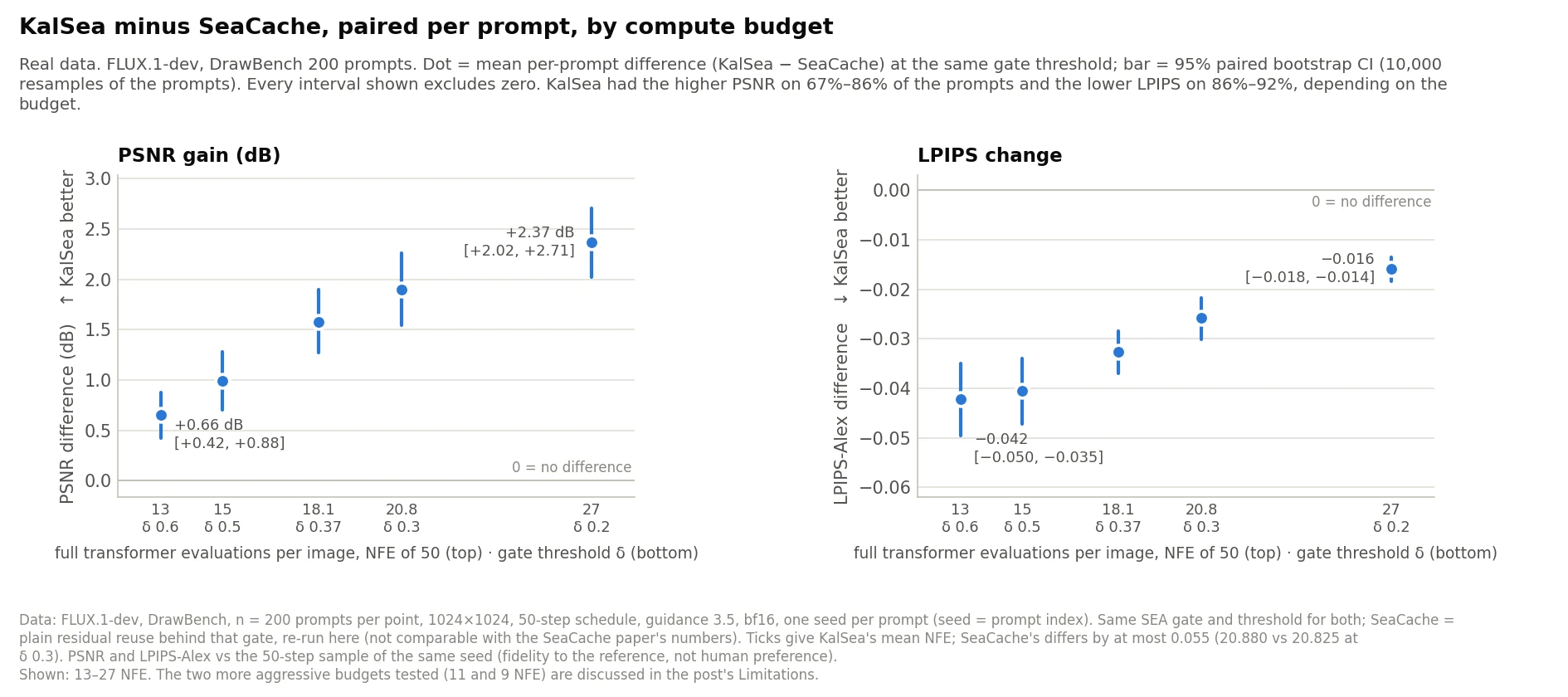
- FLUX.1-dev (DrawBench, 200 prompts, 1024², 50 steps): measured against the 50-step reference, KalSea's PSNR is +1.58 dB [+1.27, +1.90] higher than SeaCache's at 18.1 NFE (δ = 0.37) and +0.66 dB [+0.42, +0.88] higher at 13 NFE (δ = 0.6). Its LPIPS is lower by 0.033 and 0.042. KalSea is closer on 79% and 67% of prompts by PSNR and on 88% and 86% by LPIPS. Between 13 and 27 NFE the PSNR gain grows with budget, up to +2.37 dB [+2.02, +2.71] at 27 NFE, and every PSNR and LPIPS interval excludes zero. At 11 and 9 NFE the two tie in PSNR (see Limitations).
- Speed: 2.45× and 3.27× faster than the 50-step reference (5.3 s → 2.16 s and 1.62 s per image).
- FLUX.2 [dev] demo (16 prompts; a small demo with the calibration-free variant, not an evaluation): on average +4.10 dB PSNR over SeaCache at 18 of 50 evaluations and +2.12 dB at 13. KalSea has the higher PSNR on 14 and 13 of the 16 prompts.
- MiniMax-H3 demo (video with sound; a small demo with the calibration-free variant): on two of the three demo prompts (fox, waves), KalSea's video and audio are closer to the reference than SeaCache's at 23 and 14 of 49 evaluations (about 1.9× and 3× faster than the reference).
The gain comes from forecasting the block-stack residual instead of reusing it. Brackets are 95% paired bootstrap confidence intervals over prompts.
Why cache a diffusion transformer?
FLUX.1-dev [5] makes a 1024×1024 image in 50 steps, each running 19 double-stream and 38 single-stream transformer blocks over 4,096 image tokens plus the text; one image takes about 5.3 s on an NVIDIA B200. Consecutive steps are very similar, so training-free caches skip some transformer evaluations. Each cache must decide when to skip and what to write instead.
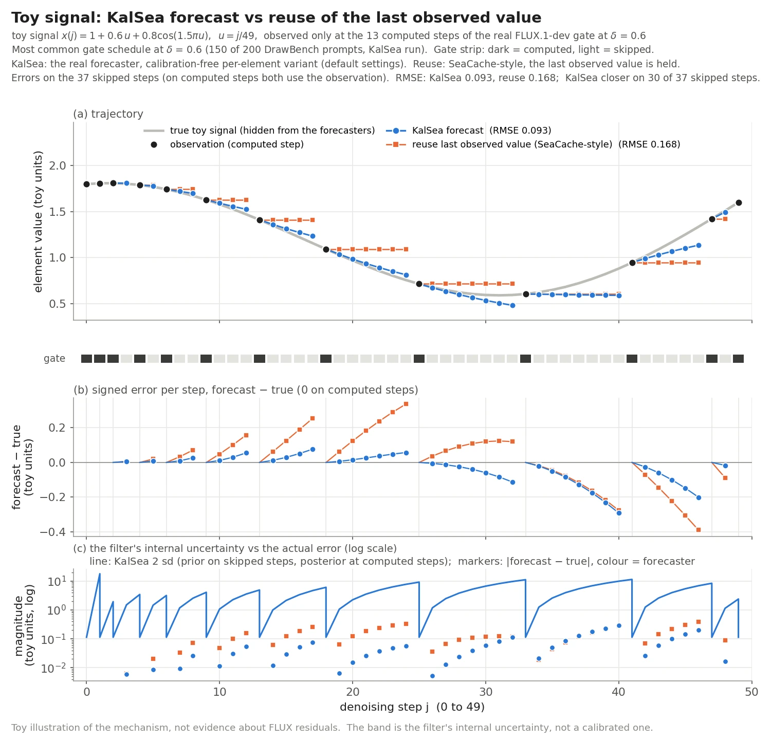
Reuse copies the last computed value. In TeaCache [3] and SeaCache [1] an adaptive gate picks the steps to compute and skipped steps reuse the cached residual. Reuse is cheap and never overshoots, but it lags behind. At δ = 0.6 the most common FLUX.1 schedule computes steps 0, 1, 2, 4, 6, 9, 13, 18, 25, 33, 41, 47, 49. Late in sampling it skips seven steps in a row, and reuse writes step 33's residual into steps 34 to 40 while the true residual keeps changing.
Forecasting predicts the skipped values from the computed ones. It can follow the drift that reuse misses, but it can also overshoot, and errors compound over long gaps.
Background: SeaCache's spectrally aligned gate
SeaCache [1] skips steps while the accumulated change of the first transformer block's input stays small, and it measures that change on an input passed through a spectral-evolution-aware (SEA) filter. Its rationale: diffusion models build images coarse to fine, so a raw feature distance mixes emerging low-frequency content with noise that is still being removed. SeaCache derives a Wiener-like gain for under a power-law image spectrum:
For a flow-matching model like FLUX, and . The exponent is β = 2 for images; SeaCache uses 3 for video. The gain is built per spatial axis, multiplied into a separable 2-D filter and normalised to mean 1. Early on it passes only the coarsest layout; as σ falls the pass band widens until the filter is flat.
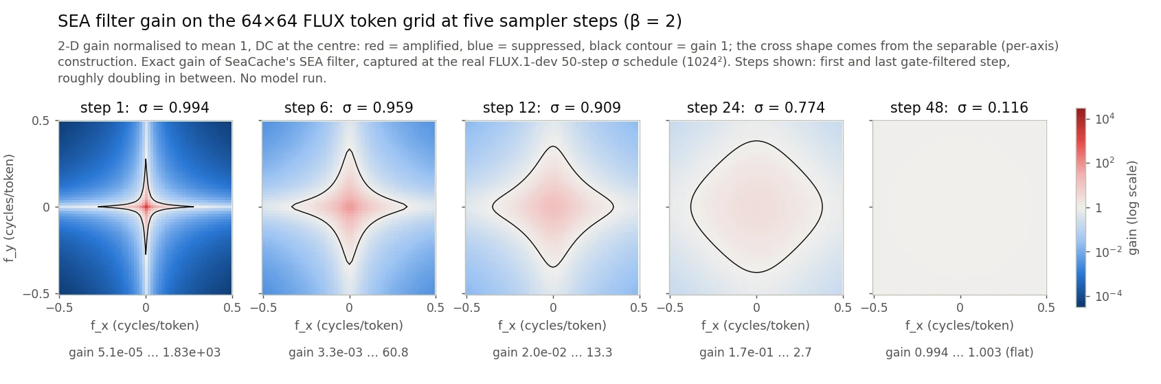
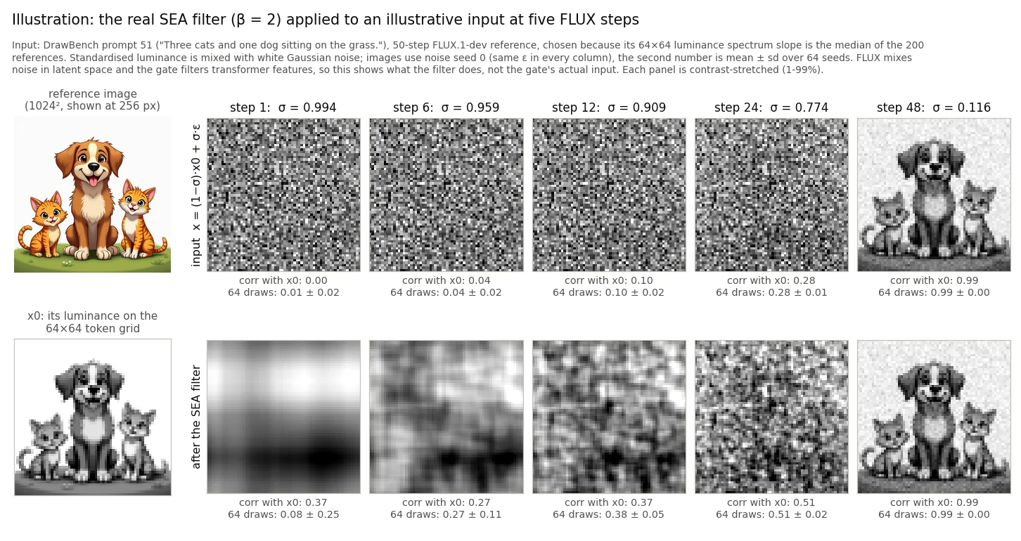
The gate rule. Filter the first block's input after its timestep-dependent AdaLN shift and scale, and add its relative L1 change to a running sum. While the sum stays below a threshold δ, skip. Otherwise run the full transformer and reset the sum. The first and last steps are always computed. On a skipped step SeaCache adds the last computed residual to the current input. This plain residual reuse is the baseline throughout this post.
On FLUX.1-dev with 50 steps, δ maps to evaluations as follows: 0.2 → 27, 0.3 → 20.8, 0.37 → 18.1, 0.5 → 15, 0.6 → 13, 0.8 → 11, 1.0 → 9.
Related work that forecasts instead of reusing includes TaylorSeer [4], which extrapolates features with finite differences, and SpecKCast [2], which forecasts the model output with one Kalman filter per DCT coefficient and lets the filter's uncertainty choose the steps. We do not compare against them.
KalSea: forecast the residual instead of reusing it
KalSea keeps SeaCache's gate to decide when to skip. For what to write on a skipped step, it replaces reuse with a forecast of the block-stack residual. The forecaster is adapted from SpecKCast and applied to the residual instead of the model output.
The skip path
On FLUX the residual is the change the 57 transformer blocks make to the image tokens, a 4,096 × 3,072 tensor (tokens × channels). At every step:
- Embed the current latent (always computed, cheap) to get the block-stack input .
- Gate: filter the first block's modulated input and add its relative L1 change to the running sum.
- Computed step (first, last, or sum ≥ δ): run all blocks to get , give the residual to the Kalman update, and reset the sum.
- Skipped step: set with the forecast . No block runs.
- Output layers always run and produce the velocity.
SeaCache's path is identical except that step 4 adds the last computed . In both, comes from the current latent; only the blocks' contribution is filled in.
The Kalman forecaster
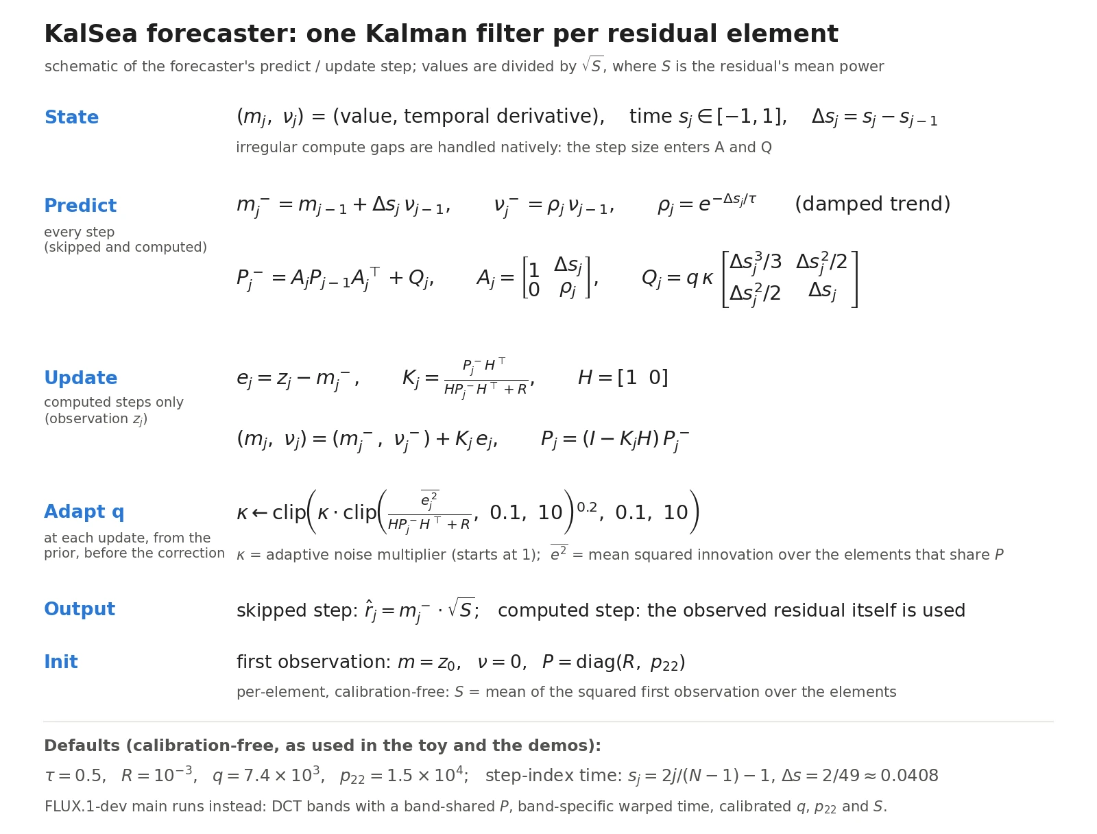
Every element of the residual has a state : a value and its temporal derivative. Time is a coordinate over the 50 steps, with step size . Values are divided by the square root of the residual's power.
Predict, at every step:
Update, on computed steps only, with the observed residual , and observation noise :
On a skipped step the forecast is , scaled back to the residual's units. The equation card below gives the full matrices. Four details matter:
- Damped trend. The derivative decays with time constant τ (KalSea 0.5; SpecKCast 0.1 for velocities), so a long gap cannot extrapolate a stale slope forever.
- Irregular schedules are native. The filter advances through skipped steps too, and enters both the transition and the process noise , so over a seven-step gap the damping compounds and the uncertainty grows.
- Fixed memory. All elements on one time axis share one 2×2 covariance. The state is two fp32 tensors the size of the residual and does not grow with the number of evaluations.
- Online process-noise adaptation (from SpecKCast): at each update the process noise is rescaled towards the observed squared innovation over its predicted variance.
Two configurations
FLUX.1 main configuration (DCT bands). Following SpecKCast, each channel's 64×64 token grid goes through an orthonormal 2-D DCT and is split into 7 radial frequency bands. Each band shares one covariance and noise level and gets its own time axis, warped by the log signal-to-noise ratio. Band powers and noise come from an offline calibration on 16 COCO prompts. In residual space the bands turn out not to matter: a calibrated per-element variant (no DCT; calibrated noise and warped time pooled over the bands) scores about the same (see Design notes). That FLUX.1 ablation is distinct from the calibration-free variant below.
Calibration-free (per-element). For a new model, the per-element filter needs no calibration file. It uses q = 7.4 × 10³ and initial trend variance = 1.5 × 10⁴ (the FLUX calibration pooled over the 7 bands), takes the signal scale from the first observation and uses uniform step-index time. The large noise values make the filter trust each observation, which is meant to make it tolerant of a model's unknown scale (untested beyond the two demos); on the toy the value gain stays above 0.996 at every update. These defaults were reasoned from the equations, not tuned. This variant runs the toy and both demos; its image quality was not evaluated on FLUX.1.
Results on FLUX.1-dev
Setup
- Model and prompts: FLUX.1-dev, bf16, 50 steps, 1024×1024, guidance 3.5, NVIDIA B200 GPUs; the 200 DrawBench prompts [7], one image each, seed = prompt index.
- Metrics: fidelity to the 50-step image of the same seed (PSNR, SSIM, LPIPS-AlexNet [9]).
- Baseline: SeaCache = plain residual reuse behind the same gate. On the 4 images we checked, our reuse path was bit-identical to the official SeaCache FLUX implementation.
- Matched compute: the same gate code and δ; only the skip path differs. Mean NFE matches to within 0.06 at every threshold shown (see the budget table).
- No tuning on the test set: τ was chosen on 64 COCO prompts [8], disjoint from DrawBench and from the 16 calibration prompts.
- Statistics: 95% paired bootstrap CIs over the 200 prompts (10,000 resamples).
Main table
| Method (what fills the skipped steps) | PSNR ↑ (18.1 NFE) | SSIM ↑ (18.1 NFE) | LPIPS ↓ (18.1 NFE) | PSNR ↑ (13 NFE) | SSIM ↑ (13 NFE) | LPIPS ↓ (13 NFE) |
|---|---|---|---|---|---|---|
| 50-step reference (50 NFE) | ∞ | 1 | 0 | ∞ | 1 | 0 |
| SeaCache: plain residual reuse | 25.33 | 0.8799 | 0.1128 | 21.26 | 0.8001 | 0.2138 |
| KalSea (main, DCT bands) | 26.91 | 0.9066 | 0.0801 | 21.91 | 0.8256 | 0.1716 |
| KalSea, per-element (calibrated, no DCT) | 26.87 | 0.9067 | 0.0799 | 21.94 | 0.8292 | 0.1693 |
Real data, all 200 DrawBench prompts, no selection. 18.1 NFE is δ = 0.37 (18 or 19 per prompt); 13 NFE is δ = 0.6 (exactly 13 per prompt). Both KalSea rows beat SeaCache in every column; the two KalSea rows are equal within noise (see Design notes). The per-element row drops only the DCT band decomposition; it keeps calibrated noise and a calibrated, band-independent warped time axis.
Paired differences, KalSea (main) minus SeaCache:
- 18.1 NFE: PSNR +1.58 dB [+1.27, +1.90], SSIM +0.0267 [+0.0227, +0.0307], LPIPS −0.0327 [−0.0370, −0.0284]. KalSea is better on 79% (PSNR), 84.5% (SSIM) and 88% (LPIPS) of prompts.
- 13 NFE: PSNR +0.66 dB [+0.42, +0.88], SSIM +0.0255 [+0.0196, +0.0315], LPIPS −0.0422 [−0.0496, −0.0349]. KalSea is better on 67%, 78.5% and 86% of prompts.
- Per-element KalSea minus SeaCache: +1.54 dB [+1.24, +1.84] and +0.68 dB [+0.40, +0.95].
- Replication: a full same-session re-run gave +1.60 dB [+1.29, +1.92] and +0.66 dB [+0.42, +0.88].
Speed
| 50-step reference | KalSea, 18.1 NFE | KalSea, 13 NFE | |
|---|---|---|---|
| latency per image | 5.295 s | 2.158 s (2.45×) | 1.618 s (3.27×) |
Real data, same-session means over 200 prompts (configurations interleaved per prompt, 5 concurrent single-GPU processes, whole pipeline call). Plain reuse at the same NFE is about 3% faster (see Limitations).
By NFE alone the speed-ups would be 2.76× and 3.85×; the gap is text encoding, VAE decoding, and the gate and output layers that run on every step (on the plain-reuse path a computed step takes about 102 ms and a skipped one about 2.5 ms; KalSea's forecast adds about 53 to 66 ms per image). KalSea's extra GPU memory over the uncached run is 0.141 GiB at both thresholds (plain reuse: 0.047 GiB, so KalSea needs about 0.1 GiB more than reuse).
Across budgets: 13 to 27 NFE
| δ | NFE | PSNR, SeaCache → KalSea | ΔPSNR [95% CI] | KalSea higher PSNR | ΔLPIPS [95% CI] | KalSea lower LPIPS |
|---|---|---|---|---|---|---|
| 0.2 | 27 | 30.52 → 32.89 | +2.37 [+2.02, +2.71] | 86% | −0.0159 [−0.0184, −0.0135] | 91.5% |
| 0.3 | 20.8 | 26.89 → 28.79 | +1.90 [+1.54, +2.26] | 82.5% | −0.0258 [−0.0301, −0.0218] | 92% |
| 0.37 | 18.1 | 25.33 → 26.91 | +1.58 [+1.27, +1.90] | 79% | −0.0327 [−0.0370, −0.0284] | 88% |
| 0.5 | 15 | 22.79 → 23.79 | +0.99 [+0.71, +1.28] | 73.5% | −0.0406 [−0.0472, −0.0340] | 87% |
| 0.6 | 13 | 21.26 → 21.91 | +0.66 [+0.42, +0.88] | 67% | −0.0422 [−0.0496, −0.0349] | 86% |
Real data, all 200 prompts at each threshold, no selection. Δ = KalSea minus SeaCache, paired per prompt. At δ = 0.3 SeaCache used slightly more evaluations (20.88 vs 20.825). The two more aggressive thresholds (11 and 9 NFE) are covered in Limitations.
Qualitative examples
The examples below are selected wins. At δ = 0.6 both methods computed the same steps on 183 of 200 prompts; KalSea's PSNR is higher on 122 of these, and on 119 of them its LPIPS is also lower. Those 119 prompts are the pool for every FLUX.1 example; their PSNR gains range from +0.004 to +4.88 dB (median +1.23). Over all 200 prompts the mean gain is +0.66 dB and the median +0.60 dB.

Design notes
τ = 0.5, not SpecKCast's 0.1. τ = 0.5 beats τ = 0.1 by +0.29 dB [+0.14, +0.46] at 18.1 NFE and by +0.17 dB [+0.02, +0.32] at 13 NFE. On the tuning set τ from 0.2 to 3 is a broad plateau (26.73 to 26.85 dB at δ = 0.37, 21.43 to 21.50 dB at δ = 0.6). Even with τ = 0.1, KalSea beats SeaCache by +1.29 dB [+1.04, +1.55] and +0.49 dB [+0.33, +0.64]. Presumably the residual evolves more smoothly than the velocity SpecKCast forecasts (untested).
Per-element ≈ DCT bands. Per-element minus DCT is −0.04 dB [−0.12, +0.04] at 18.1 NFE and +0.02 dB [−0.14, +0.18] at 13 NFE. The LPIPS differences are not significant either; SSIM is equal at 18.1 NFE and slightly favours per-element at 13 NFE (+0.004 [+0.0005, +0.007]). The DCT bands do not help in residual space, so none of the gain should be credited to them. The spectral component with evidence behind it is SeaCache's gate (SeaCache's own ablation; we did not ablate it).
NFE is matched; step positions are not always identical. The gate reads each method's own trajectory. KalSea computes the same steps as SeaCache on 192 of 200 prompts at δ = 0.37, 183 at δ = 0.6, and 178 to 199 across the five thresholds in the budget table. The comparison is matched in compute, not step for step.
Demo: FLUX.2 [dev]
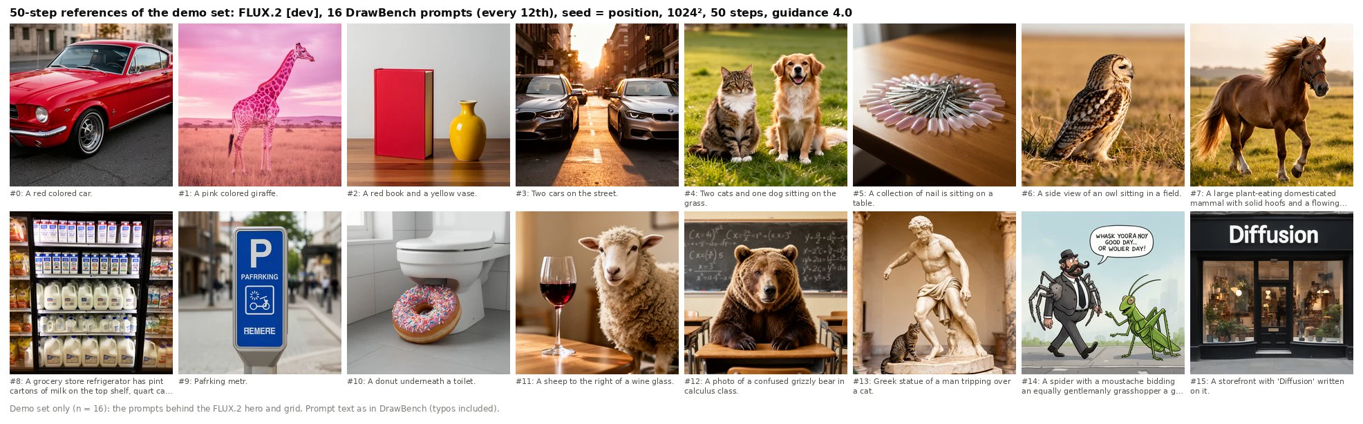
A small demo (16 prompts, one seed each), not an evaluation, with the calibration-free, per-element KalSea rather than the calibrated DCT variant from the FLUX.1 tables.
The port. FLUX.2 [dev] [5] has 8 double-stream and 48 single-stream blocks at width 6144, with AdaLN modulations computed once per forward pass and shared across blocks. Its single-stream blocks run over the concatenated text and image tokens, so the residual is taken on the image rows only. The gate reads the first double block's modulated image input and must use the scheduler's float32 σ; σ read from the bf16 timestep collapsed the gate distance (fixed before any real run).
Setup. Every 12th DrawBench prompt, seed = position 0 to 15, 1024², 50 steps, guidance 4, configurations interleaved per prompt. FLUX.2's σ schedule differs, so 18 and 13 evaluations need δ = 0.47 and 0.8. SeaCache and KalSea computed identical steps on all 16 prompts at both. In this section #k is the position in the 16-prompt subset (DrawBench prompt 12k), not the DrawBench index used for FLUX.1.
| 16 prompts | PSNR ↑ (18) | SSIM ↑ (18) | LPIPS ↓ (18) | PSNR ↑ (13) | SSIM ↑ (13) | LPIPS ↓ (13) |
|---|---|---|---|---|---|---|
| SeaCache reuse | 23.78 | 0.8889 | 0.0996 | 20.12 | 0.8191 | 0.1738 |
| KalSea, calibration-free | 27.88 | 0.9278 | 0.0527 | 22.24 | 0.8633 | 0.1204 |
| KalSea − SeaCache | +4.10 [+2.51, +5.82] | +0.039 [+0.026, +0.053] | −0.047 [−0.075, −0.028] | +2.12 [+0.70, +3.44] | +0.044 [+0.023, +0.068] | −0.053 [−0.083, −0.028] |
| KalSea better on | 14 / 16 | 15 / 16 | 15 / 16 | 13 / 16 | 14 / 16 | 14 / 16 |
Demo data, all 16 prompts, no selection; 18 (δ = 0.47) and 13 (δ = 0.8) of 50 evaluations. Fidelity to the same-session 50-step reference. KalSea took 5.81 s (2.67× faster than the reference's 15.49 s) at 18 and 4.27 s (3.63×) at 13 evaluations; plain reuse at the same evaluations is slightly faster (see Limitations). With n = 16 the intervals are indicative only.
The margins are larger than on FLUX.1, but with different prompts, n = 16 and a different variant that is at most a hint.

Demo: MiniMax-H3, video with sound
A small demo, not an evaluation, again with the calibration-free per-element KalSea.
The port. MiniMax-H3 [6] runs one 50-block transformer over a packed sequence of text, audio and video tokens, one forward pass per step. The gate filters the first block's modulated video input on its (frames, height, width) grid with SEA exponent 3, SeaCache's value for video. Video and audio rows each get their own Kalman forecaster on the video gate's schedule; the text rows, which the output heads never read, are not computed on skipped steps.
Setup. Three prompts with sound, one seed each: 960×544, 124 frames (5.2 s), 49 evaluations for the reference (the first 3 steps and the last are always computed), one B200 per run without offloading. For the SeaCache baseline both forecasters were replaced by a copy of the last residual, gate and forward pass unchanged. Plain H3 is deterministic (a repeated reference run gave a bitwise-identical video and an audio track at over 300 dB SNR), so the differences come from the cache. δ = 0.3 gives 23 evaluations and δ = 0.6 gives 14, with identical computed steps for SeaCache and KalSea in every run. Shown here are the 2 of the 3 prompts where KalSea's video and audio both beat SeaCache's at both thresholds: a fox trotting through snow (seed 42) and waves on volcanic rocks (seed 43). On the third, SeaCache's video was closer (see Limitations).
| prompt | δ (evaluations) | video PSNR, SeaCache / KalSea | frames where KalSea is closer | audio SNR, SeaCache / KalSea | KalSea latency (speed-up) |
|---|---|---|---|---|---|
| fox | 0.3 (23) | 29.52 / 30.39 | 109 / 124 | 8.20 / 14.30 | 37.3 s (1.87×) |
| fox | 0.6 (14) | 24.86 / 26.52 | 101 / 124 | 2.62 / 5.44 | 23.3 s (2.99×) |
| waves | 0.3 (23) | 34.12 / 36.88 | 124 / 124 | 10.05 / 14.07 | 35.9 s (1.93×) |
| waves | 0.6 (14) | 28.32 / 29.40 | 124 / 124 | 4.53 / 7.64 | 23.1 s (3.00×) |
Demo data, one run per cell, dB against the 49-evaluation reference; bold = closer. Selection: 2 of the 3 demo prompts (see Limitations for the third). Video: mean per-frame PSNR over 124 lossless frames. Audio: stereo waveform SNR (phase-sensitive, not perceptual); STFT-magnitude SNR agrees in all four rows. Latency: whole call, one timed run, vs the reference's 69.6 s (fox) and 69.5 s (waves); SeaCache ran in a later session, so its latency is not compared.
At δ = 0.6 KalSea's waveform SNR is low (5.4 dB fox, 7.6 dB waves), though above SeaCache's (2.6 and 4.5 dB). The spectrograms stack the reference, SeaCache reuse and KalSea at both thresholds. By eye, the fox spectrograms show some snow-crunch transients smeared at δ = 0.6, more visibly for SeaCache, while the video stays close. The waves spectrograms show no clear damage. There was no listening test.
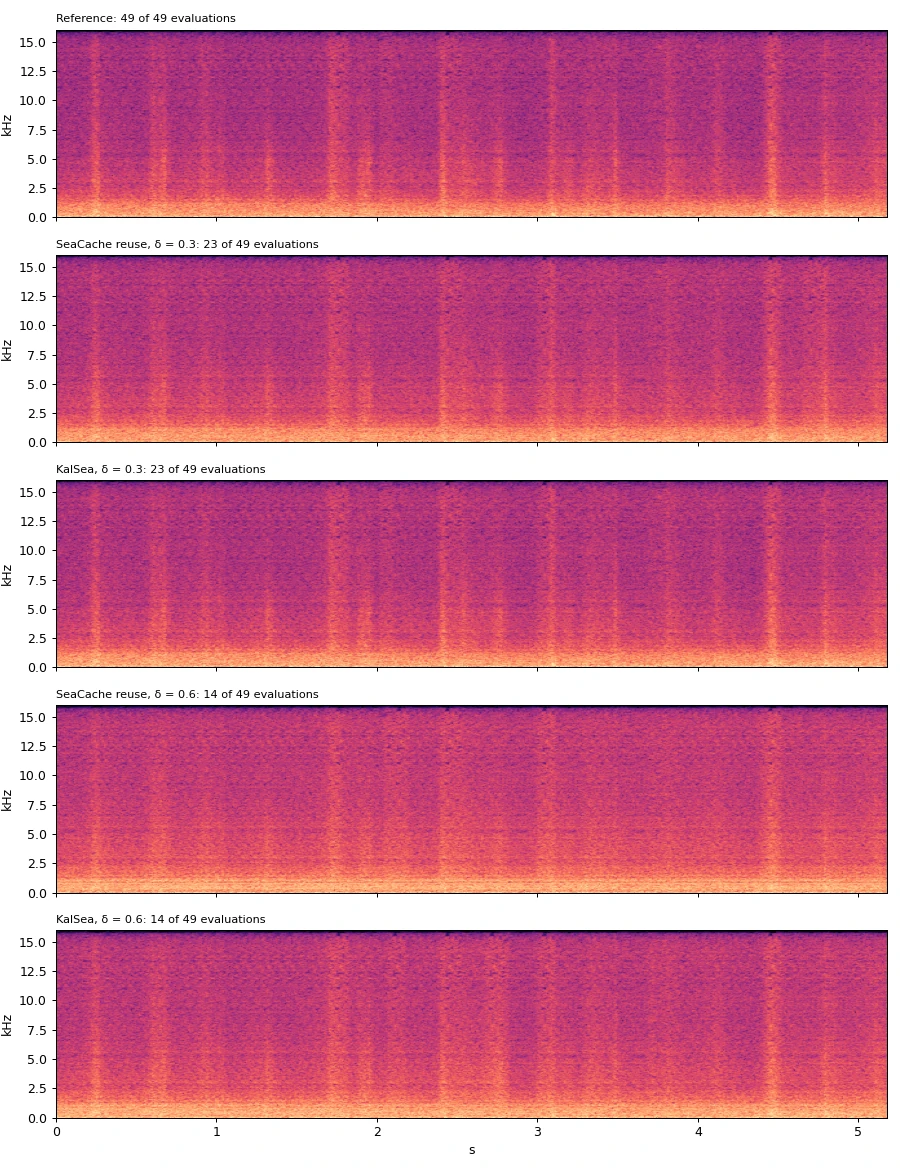
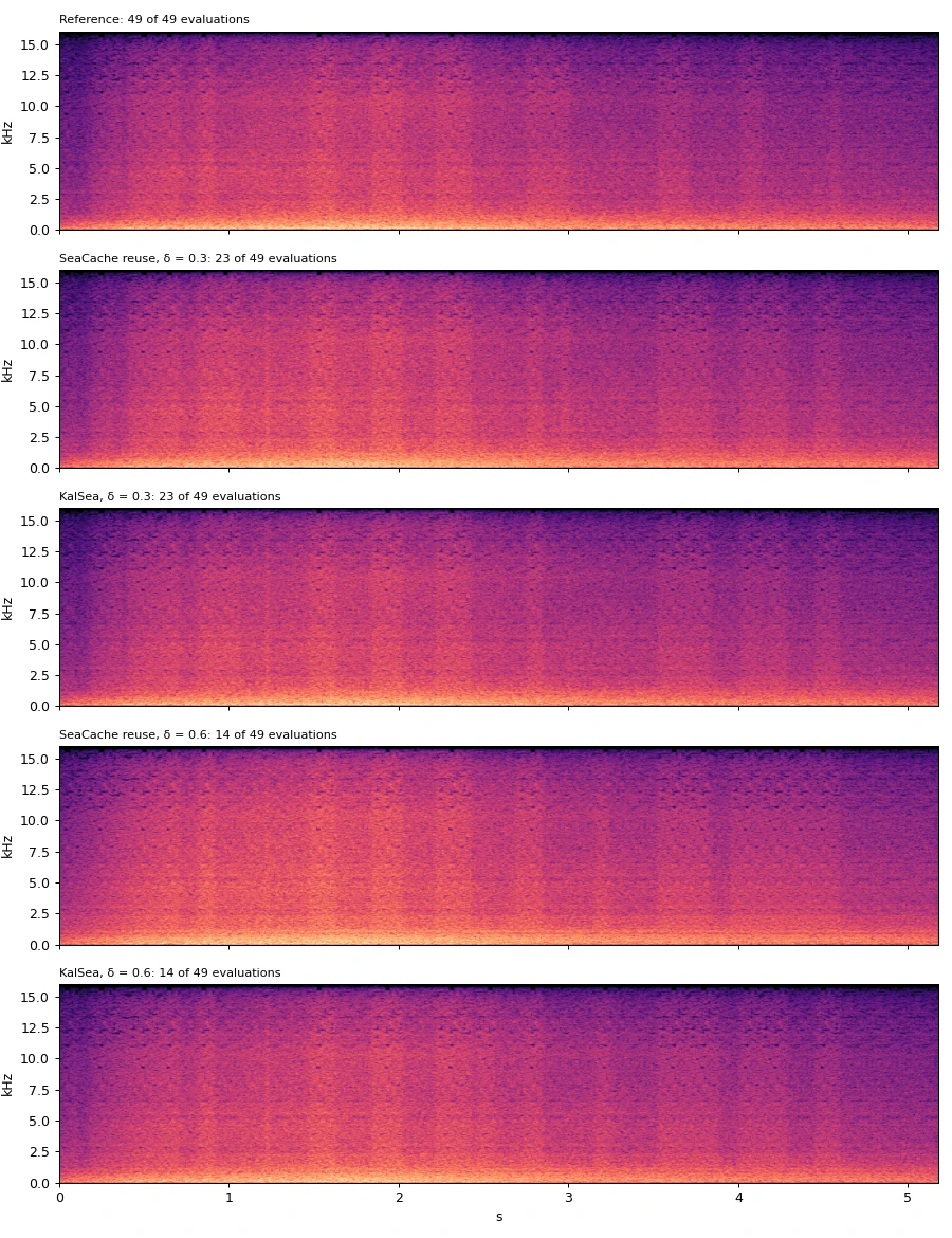
Demo data, 5.2 s with sound. Selection: the 2 of 3 demo prompts where KalSea's video and audio beat SeaCache's at both thresholds; on the third, SeaCache's video was closer at both. Each video has three soundtracks: KalSea (default), SeaCache reuse, reference. Browsers usually play only the first; switch tracks in a player such as VLC or mpv, or play the separate soundtracks below.
| soundtrack | reference | SeaCache reuse | KalSea |
|---|---|---|---|
| fox, δ = 0.3 (23 of 49) | |||
| fox, δ = 0.6 (14 of 49) | |||
| waves, δ = 0.3 (23 of 49) | |||
| waves, δ = 0.6 (14 of 49) |
Demo data, same 2 of 3 prompts. AAC copies of the soundtracks in the videos above.
Limitations
- FLUX.1-dev (200 DrawBench prompts, one seed each) is the only evaluation. FLUX.2 [dev] (16 prompts) and MiniMax-H3 (3 prompts) are small demos run with the calibration-free variant, which was not evaluated on FLUX.1.
- At the most aggressive FLUX.1 budgets tested (11 and 9 of 50 evaluations), KalSea and SeaCache are tied in PSNR (+0.11 dB [−0.14, +0.34] and −0.10 dB [−0.31, +0.10]); KalSea still has the lower LPIPS.
- On one of the three MiniMax-H3 demo prompts, SeaCache's video was closer to the reference.
- At the same number of evaluations, KalSea adds about 3% wall-clock time and about 0.1 GiB GPU memory over plain reuse.
- KalSea runs are not bit-reproducible: a re-run with the same configuration and seed gave bit-identical images on only 6 of 200 prompts at δ = 0.37, although mean PSNR moved by only 0.02 dB (reuse was bit-identical on all 200).
- Fidelity to the 50-step reference is not human preference.
- Our SeaCache numbers come from our own re-run and are not comparable with the numbers in the SeaCache paper. For example, here δ = 0.3 gives 20.8 of 50 evaluations, while the paper reports 37% of full TFLOPs at δ = 0.3 on FLUX.
- We compare only against plain reuse at the same gate, so we make no claim that a Kalman filter beats other forecasters.
- Latency was measured with concurrent single-GPU processes and depends on load; NFE is the hardware-independent budget.
References
- J. Chung, S. Hyun, M. Lee et al. SeaCache: Spectral-Evolution-Aware Cache for Accelerating Diffusion Models. CVPR, 2026. Code: github.com/jiwoogit/SeaCache. The gate, the SEA filter and its rationale; its plain residual reuse is our baseline.
- J. Rajabi, H. C. Karaimer, D. B. Lindell et al. SpecKCast: Spectral Kalman Forecasting for Diffusion Acceleration. arXiv:2610.26837, 2026. Source of KalSea's Kalman forecaster: damped trend, shared covariance, online process-noise adaptation, DCT bands and band-specific time warp.
- F. Liu, S. Zhang, X. Wang et al. Timestep Embedding Tells: It's Time to Cache for Video Diffusion Model (TeaCache). CVPR, 2025.
- J. Liu, C. Zou, Y. Lyu et al. From Reusing to Forecasting: Accelerating Diffusion Models with TaylorSeers. arXiv:2503.06923, 2025.
- Black Forest Labs. FLUX.1 [dev] and FLUX.2 [dev]. Model weights, run with Hugging Face Diffusers.
- MiniMax. MiniMax-H3. Model weights under the MiniMax-H3 Community License.
- C. Saharia, W. Chan, S. Saxena et al. Photorealistic Text-to-Image Diffusion Models with Deep Language Understanding (DrawBench). NeurIPS, 2022.
- T.-Y. Lin, M. Maire, S. Belongie et al. Microsoft COCO: Common Objects in Context. ECCV, 2014. COCO captions for the calibration and tuning prompts.
- R. Zhang, P. Isola, A. A. Efros et al. The Unreasonable Effectiveness of Deep Features as a Perceptual Metric (LPIPS). CVPR, 2018. PSNR and SSIM from scikit-image.
KalSea builds on ReSPect, our earlier work on residual-space forecasting.