 Prodia
One LoRA, any step count: a fast FLUX.3 Klein with AnyFlow
FLUX.3 Klein Base [1] is a strong open image model, but it samples with 50 Euler steps and classifier-free guidance (CFG), so every image costs 100 transformer passes. Most distillation methods trade this for a model that works at one fixed step count; BFL's own distilled Klein runs at 16 steps. We wanted one set of weights that works at 1, 2, 4, 8 or 16 steps, so speed and quality can be traded off per request.
We adapted AnyFlow [2], a recipe for any-step video models, to text-to-image: a single rank-256 LoRA on FLUX.3 Klein Base, trained in two stages (flow-map distillation, then on-policy distribution matching). This post covers the maths, the results with their trade-offs, and a numerical bug that broke our first attempt.
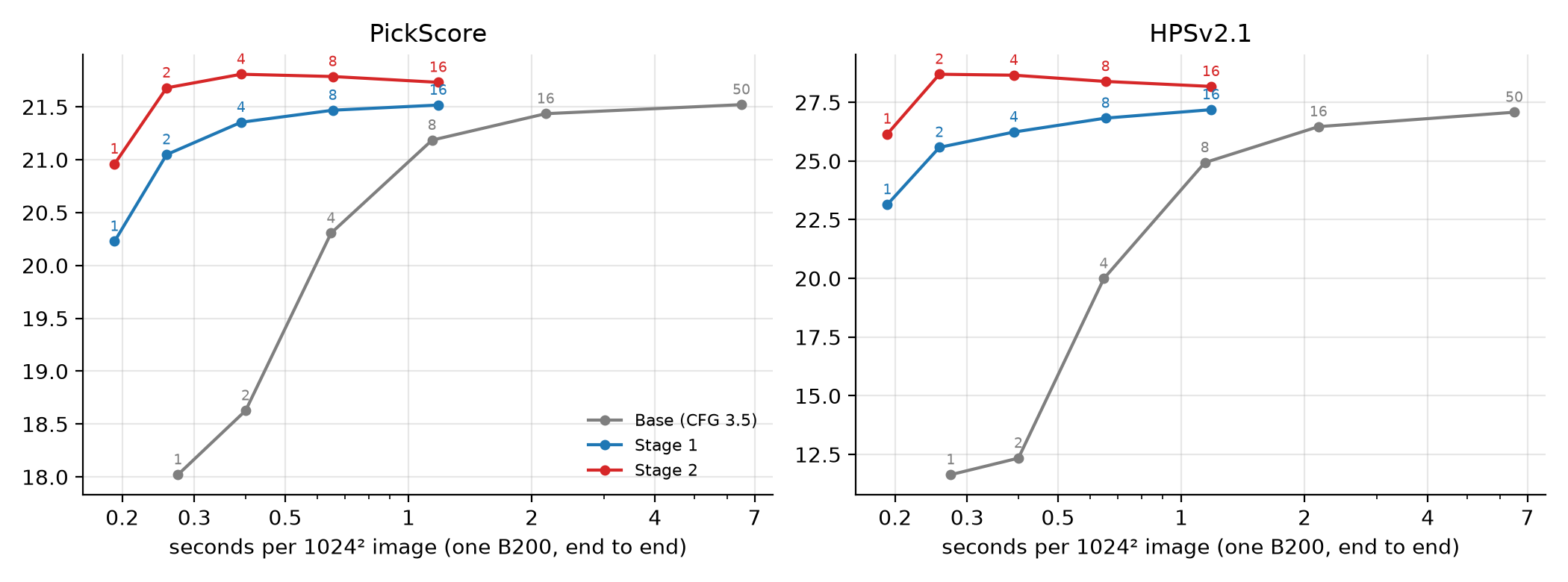
- 4 steps: 0.39 s per 1024² image vs 6.5 s for Base (one B200, end to end), 17× faster. 1 step takes 0.19 s.
- From 2 steps on, it matches or beats 50-step Base on PickScore, HPSv2.1 and CLIP (128 held-out prompts × 4 seeds).
- One checkpoint covers every step count; more steps keep the composition and refine details.
- Trade-offs: less variety between seeds (a known side effect of DMD) and more saturated colours at 1–2 steps.
Background: from velocities to flow maps
FLUX is a flow-matching model [3]. A clean latent and Gaussian noise are mixed linearly,
and the network learns the velocity . Sampling integrates the ODE from noise () to image () with Euler steps on a shifted grid:
The shift spends most of the budget at high noise: with the grid is . CFG evaluates the network twice per step, with .
Few steps fail because is only the instantaneous direction. A large Euler step cuts across the curved trajectory, and the result is blurry (Base at 1–4 steps below). A flow map learns the jump itself. The exact map moves to along the ODE and satisfies and [4]. Following MeanFlow [5], AnyFlow parameterises it with the average velocity over the interval:
Two special cases make this any-step. At , is the ordinary velocity, so the model is still a flow-matching model. At , one evaluation jumps straight to the image. Sampling with steps means jumps along the grid above, at one network pass each.
The integral is unknown, but multiplying by and differentiating in (with fixed and moving along the ODE) gives an identity that only involves the model itself:
Method
Stage 1: distil the flow map (4,000 steps)
The student is Base plus a LoRA and a new -embedding. Its regression target replaces with the CFG velocity of the frozen Base model, . This bakes guidance in, so the student needs one pass per step instead of two. The total derivative is estimated by a central difference along , which costs two extra forward passes and no Jacobian-vector product [6]:
The latents come from Base's own samples: 51,355 images at 1024² from a 56,503-prompt pool (Pick-a-Pic v2, DrawBench, T2I-CompBench, DPG-Bench), with another 2,973 prompts held out for evaluation. The details that matter, mostly from the AnyFlow paper:
- Time pairs. and for uniform . Half of the global batch is then set to (plain velocity matching) and a quarter to (one-step jumps), and both times go through . About 80% of draws land at , the region the shifted sampler actually visits.
- Weights. , the Beta(2, 1.5) shape the paper found best. The adaptive weight rescales every sample to the average loss .
- -conditioning. FLUX.3's own flow-map architecture adds the two time embeddings,
vec = time_in(t) + ref_time_in(r). We zero the output layer ofref_time_in, so the student starts out exactly equal to Base. AnyFlow's video models interpolate the two embeddings instead.
Stage 2: correct its own mistakes (1,200 steps)
Stage 1 imitates the teacher's trajectories, but at test time the model follows its own few-step path, and its errors compound. Stage 2 trains on those rollouts (on-policy). AnyFlow's backward simulation shortens any -step rollout to three flow-map jumps, which the composition property allows, and back-propagates through all three:
The sample is scored with distribution matching distillation (DMD) [7]. It is re-noised to a random level, and two models predict the clean image : the frozen Base with CFG (the "real" score) and a "fake" score, a second LoRA trained by flow matching on the generator's samples. The update pushes from the fake prediction towards the real one:
This is a reverse-KL gradient. It fixes errors on the model's own outputs, but it is mode-seeking, which shows up below as reduced diversity. The stage-1 loss stays on as co-training so the model remains a flow map. To fit in memory, the real and fake scores share one copy of Base (the fake LoRA is switched off for the real score); peak memory is 168 GB of a B200's 183 GB.
Setup and cost
| Setting | Value |
|---|---|
| Base model | FLUX.3 Klein Base: 5.5B-parameter DiT (5 per-modality + 28 shared blocks), Qwen3-VL text encoder, 16× VAE (4,096 tokens at 1024²) |
| Trainable | rank-256 LoRA on every DiT linear layer, plus ref_time_in: 603M parameters |
| Teacher data | 51,355 Base images (50 steps, CFG 3.5): 12 h, plus 2.6 h of latent and text caching |
| Stage 1 | 4,000 steps, global batch 32, lr 5e-5, EMA 0.999: 4.9 h |
| Stage 2 | 1,200 steps, global batch 32, lr 2e-6, Adam β = (0, 0.999), EMA 0.99: 4.2 h |
| Hardware | one node with 8× B200, about 24 h (≈ 190 GPU-hours) end to end |
Results
Protocol. 128 held-out prompts (never used in training), 4 seeds each, and the same initial noise for every model and step count. We report two human-preference models, PickScore and HPSv2.1 [8], and CLIP score for prompt alignment. Closeness between images is measured with LPIPS and DINOv2 [8]. Error bars are 95% bootstrap intervals over prompts.
One checkpoint, any step count
Examples
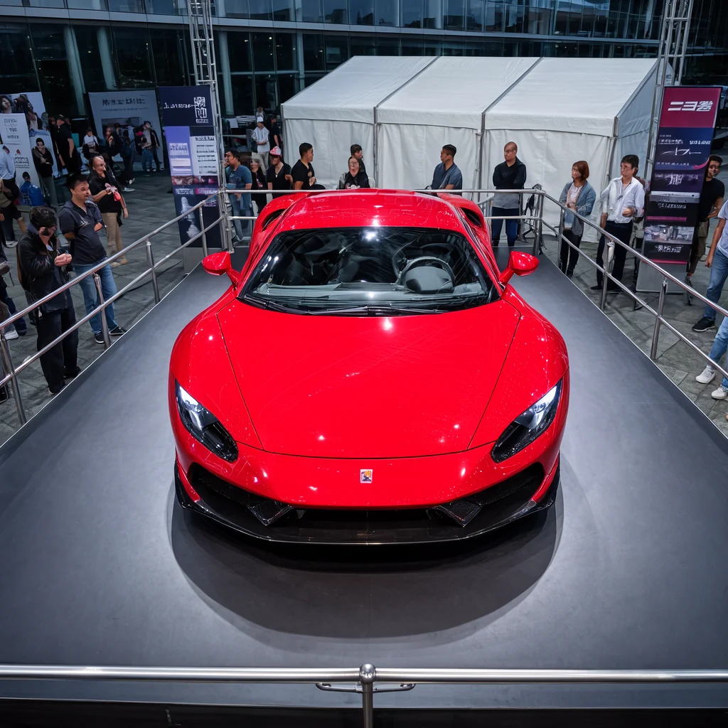
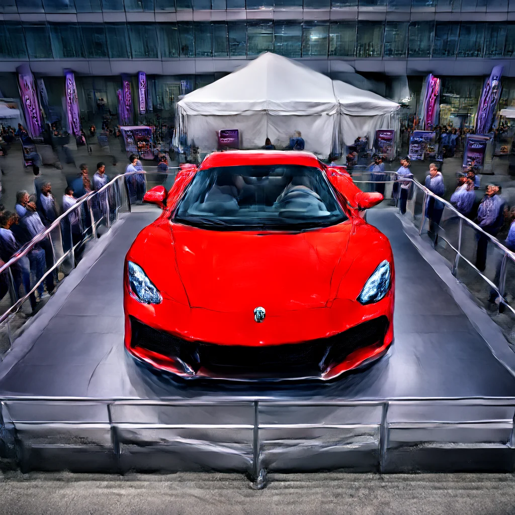
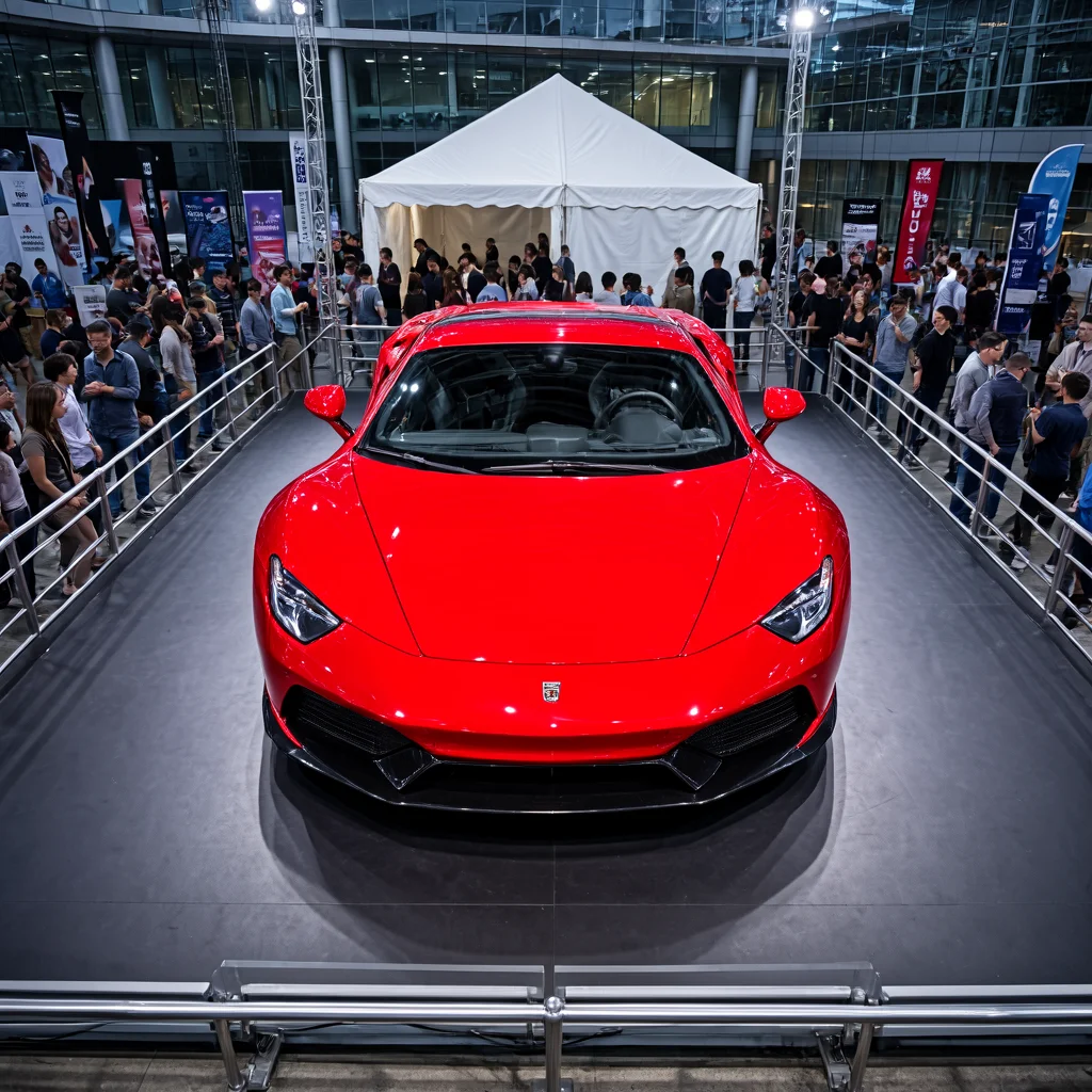
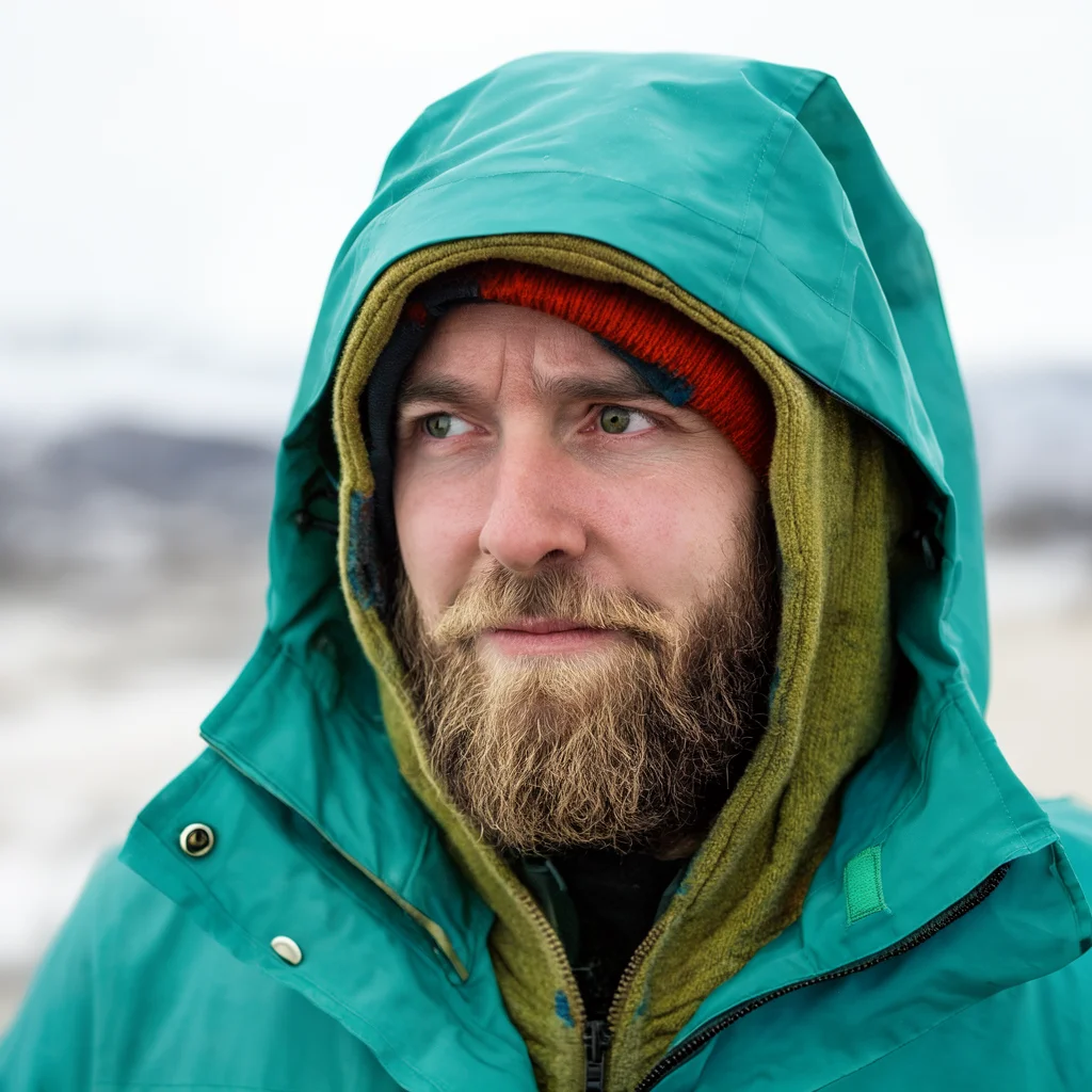
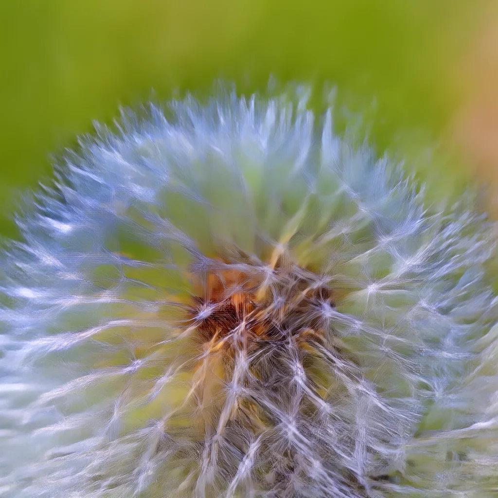
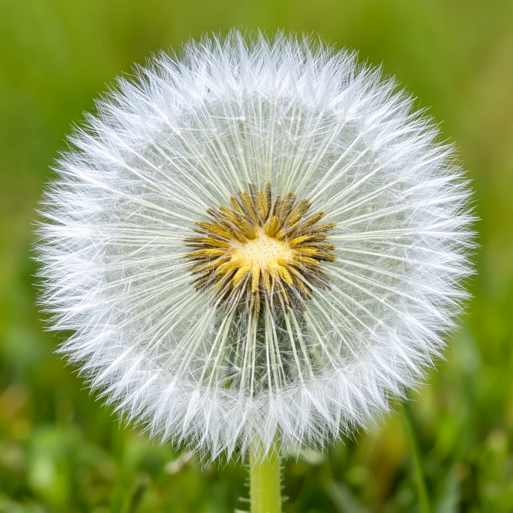
Held-out prompts, full 1024×1024 images. Base's 4 steps cost 8 network passes because of CFG.
| Prompt | Base, 4 steps | Base, 50 steps | Ours, 1 step | Ours, 4 steps |
|---|---|---|---|---|
| A sign that says “awesome” | 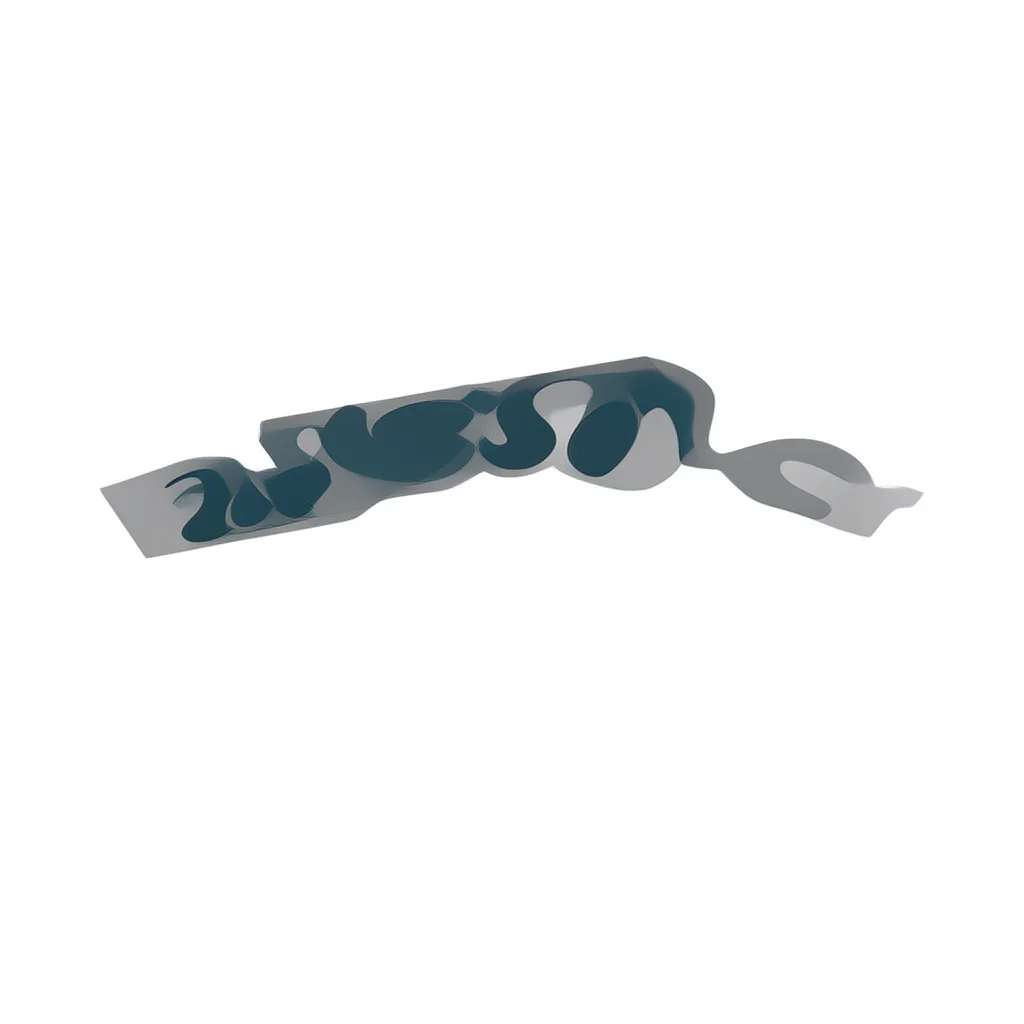 |
 |
 |
 |
| A sleek red sports car on a raised platform under bright lights … | 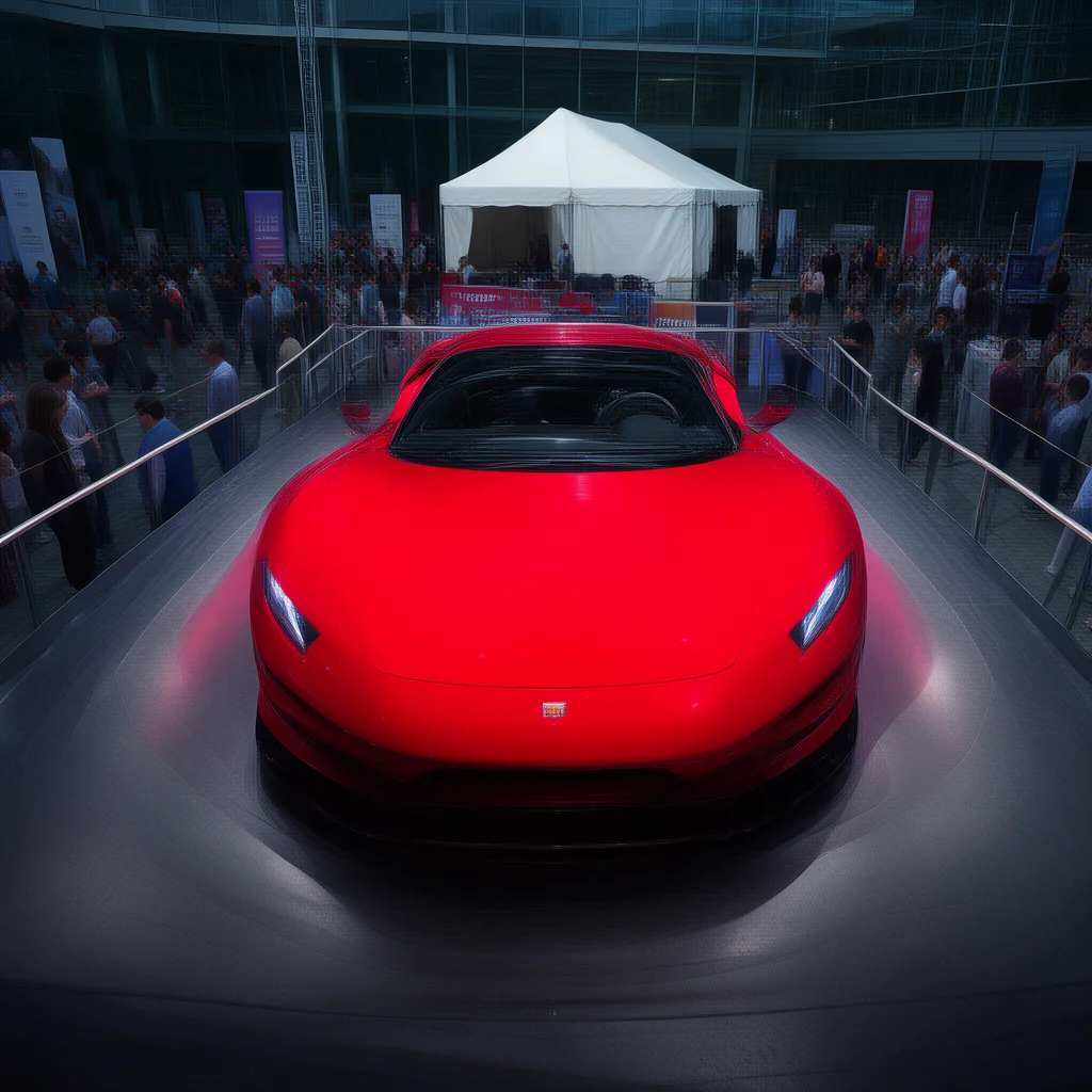 |
 |
 |
 |
| A bearded man in a hooded waterproof jacket, Iceland | 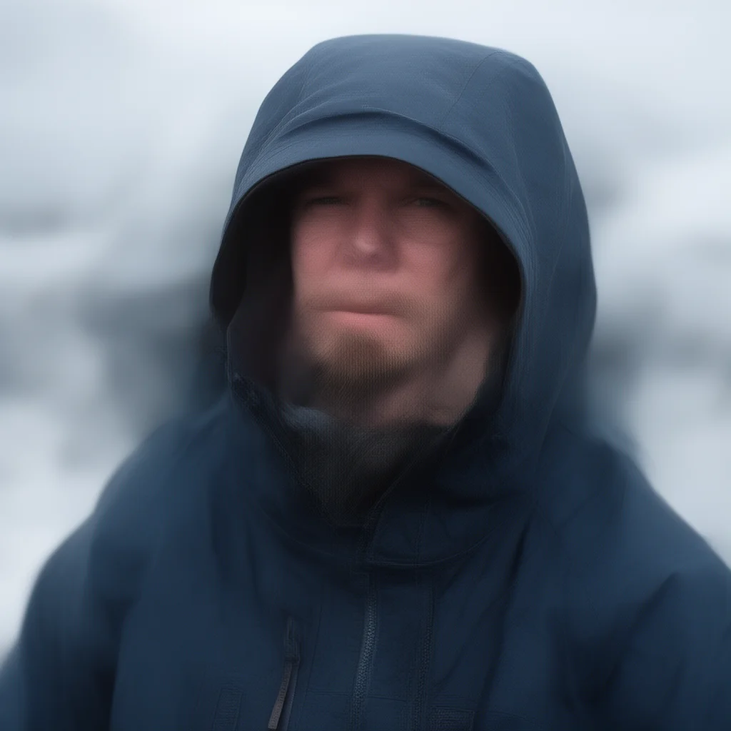 |
 |
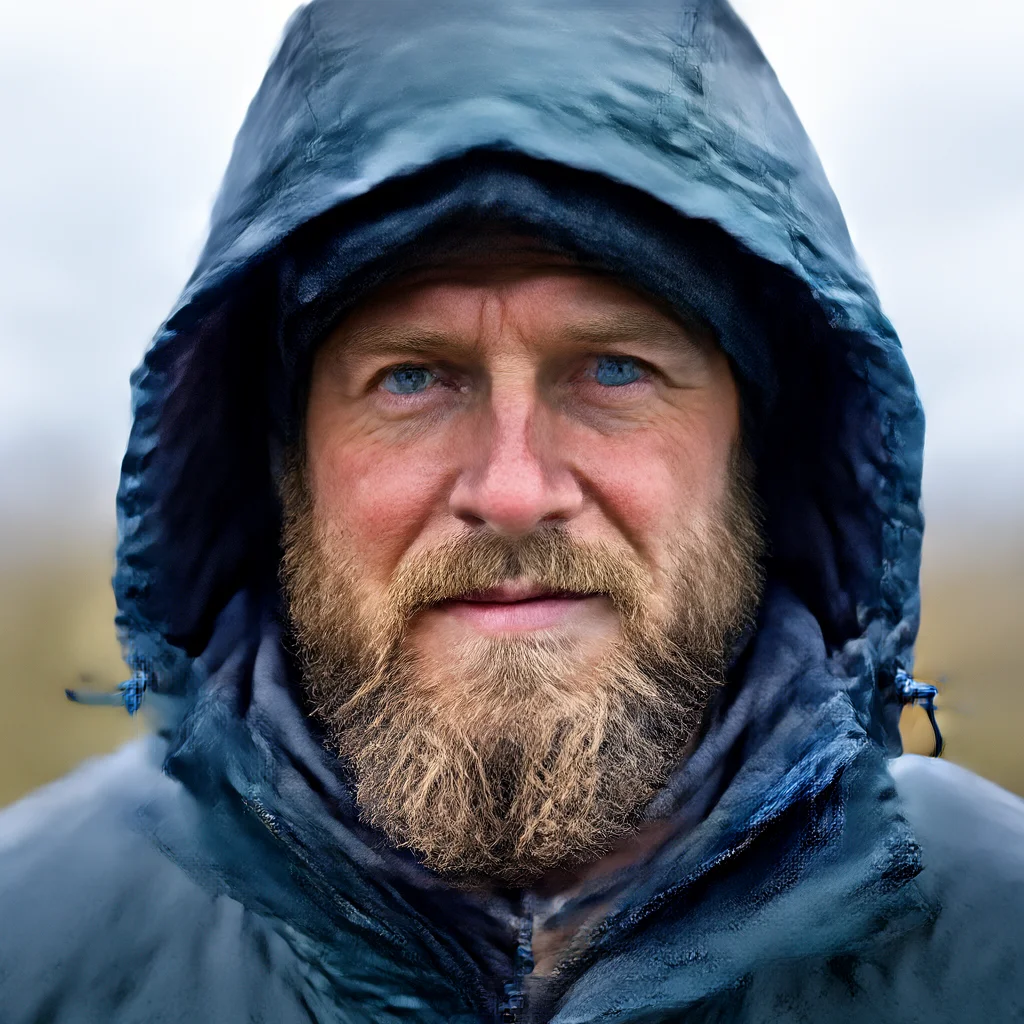 |
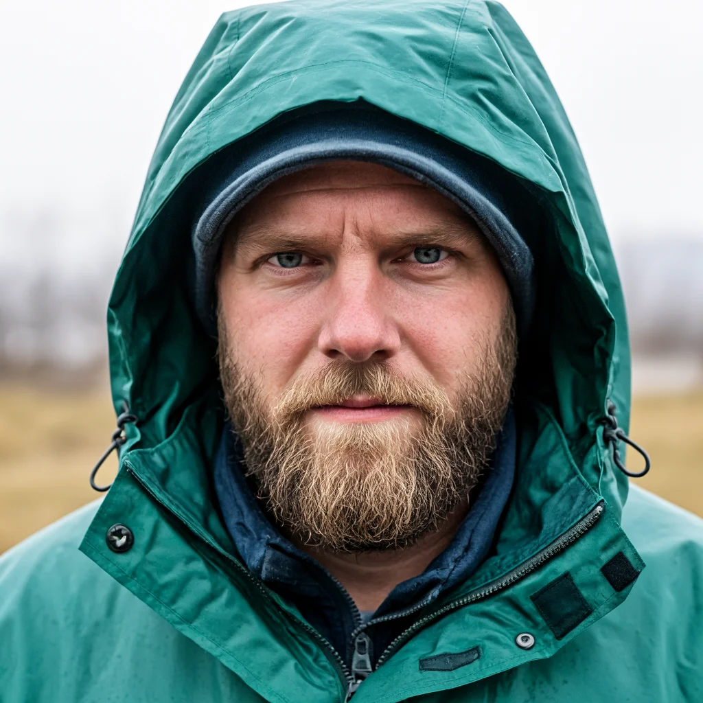 |
| macro photography of a dandelion poof | 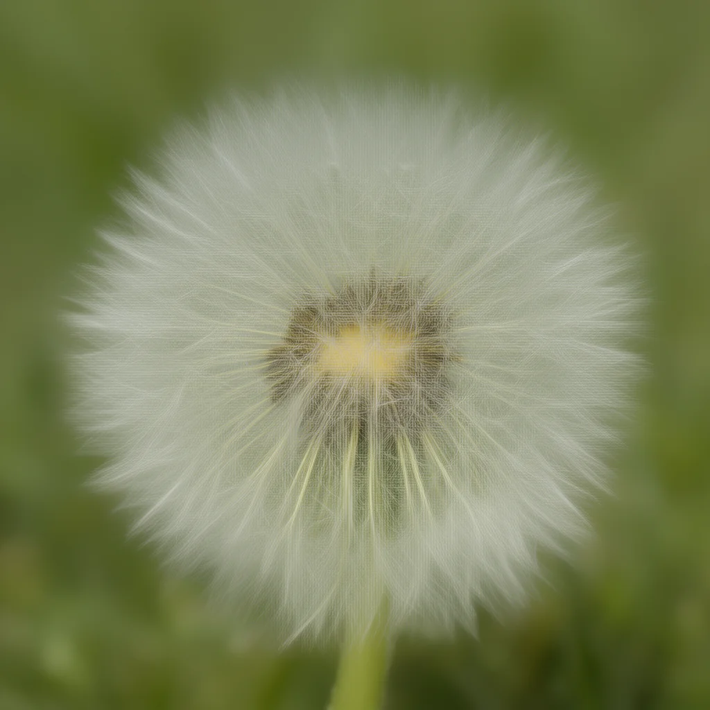 |
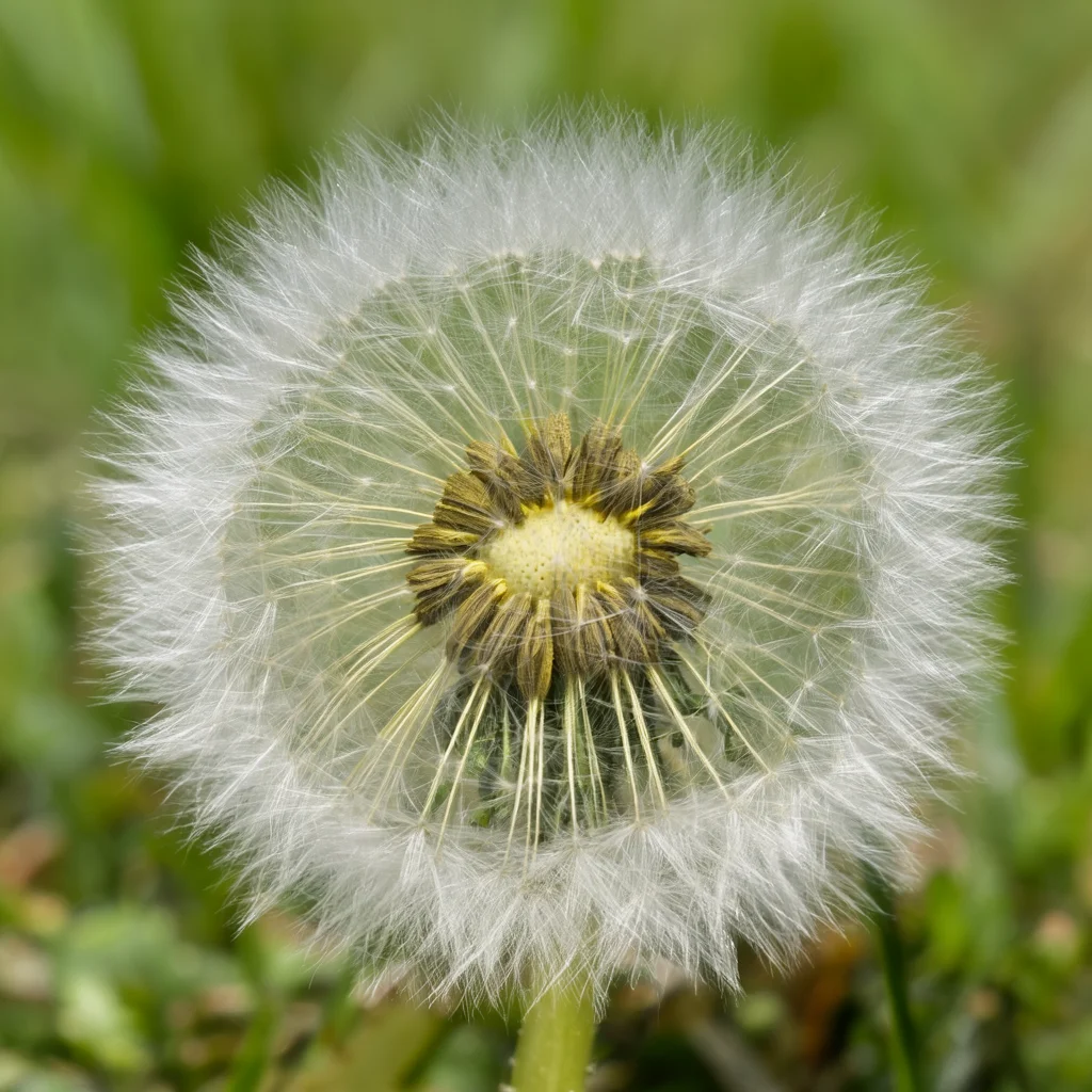 |
 |
 |
Quality vs compute
Time is end to end on one B200 (bf16, batch 1, text encoder and VAE decoder included, LoRA merged into the weights).
| Model | Steps | Network passes | Time / image | PickScore ↑ | HPSv2.1 ↑ | CLIP ↑ |
|---|---|---|---|---|---|---|
| Base + CFG | 50 | 100 | 6.50 s | 21.52 | 27.08 | 27.40 |
| Base + CFG | 8 | 16 | 1.14 s | 21.19 | 24.93 | 27.35 |
| Base + CFG | 4 | 8 | 0.65 s | 20.31 | 19.99 | 26.29 |
| Stage 1 | 1 | 1 | 0.19 s | 20.23 | 23.15 | 26.22 |
| Stage 1 | 4 | 4 | 0.39 s | 21.35 | 26.23 | 27.03 |
| Stage 1 | 16 | 16 | 1.18 s | 21.52 | 27.19 | 26.93 |
| Stage 2 | 1 | 1 | 0.19 s | 20.96 | 26.15 | 27.48 |
| Stage 2 | 2 | 2 | 0.26 s | 21.68 | 28.70 | 27.76 |
| Stage 2 | 4 | 4 | 0.39 s | 21.81 | 28.65 | 27.56 |
| Stage 2 | 16 | 16 | 1.18 s | 21.73 | 28.18 | 27.19 |
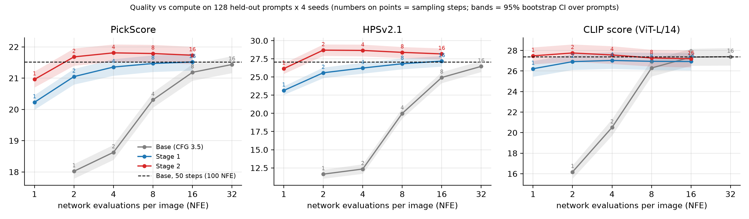
- Base needs about 16 network passes (8 steps) to stop being blurry. Stage 2 is above 50-step Base from 2 passes on.
- Paired comparison against 50-step Base on the same noise. Absolute scores vary a lot between prompts, so per-prompt differences are the fairer test. At 4 steps, Stage 2 has the higher PickScore on 73% of prompts and the higher HPSv2.1 on 84%. CLIP is a tie (+0.16, interval −0.07 to +0.39).
- Stage 1 improves steadily with more steps, the test-time scaling a flow map should have. At 16 steps it is tied with 50-step Base on PickScore (−0.00 ± 0.05) and HPSv2.1 (+0.11 ± 0.17) with 6× fewer passes, though 0.5 lower on CLIP. Stage 2 peaks at 4 steps and dips slightly after (PickScore 21.81 → 21.73): on-policy training tuned it for the few-step regime.
- Read the scores with care. Preference models reward vivid, high-contrast images, which DMD tends to produce. "On par with Base" is the fair reading, not "better".
Closeness to Base, diversity and colour
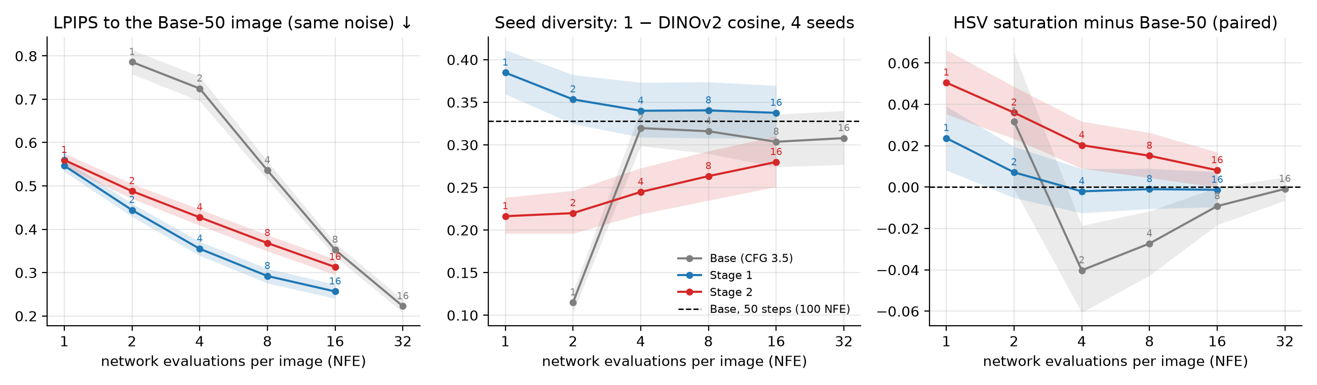
- Stage 1 follows the teacher; Stage 2 drifts to its own mode. From the same noise, Stage 1 lands closer to Base's own image than Stage 2 at every step count (LPIPS 0.26 vs 0.31 at 16 steps). Stage 1 imitates trajectories, while DMD only matches the overall distribution.
- Diversity drops in Stage 2. The DINOv2 distance between seeds is 0.33 for 50-step Base and 0.34 for Stage 1 at 4 steps, but 0.22–0.25 for Stage 2 at 1–4 steps, and lower than Base on 87% of prompts. More steps bring some of it back (0.28 at 16). This is the mode-seeking side of reverse KL, shown in the video below.
- Colour is more saturated at few steps. Stage 2's saturation is 18% above Base at 1 step, falling to 3% at 16. The AnyFlow paper warns that a zero-initialised -embedding can grow during training and over-saturate images. We checked our additive embedding on the sampling grids. For the intermediate jumps, the conditioning vector stays within 2% of Base's norm, but the final jump to is 23% larger with 4 steps and 38% larger with 1 step. That ordering matches the saturation shift; it's suggestive, not proven.
Where it differs from Base
| Prompt | Base, 50 steps | Ours, 1 step | Ours, 4 steps | Note |
|---|---|---|---|---|
| four pigs and three plates | 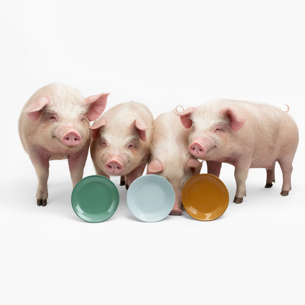 |
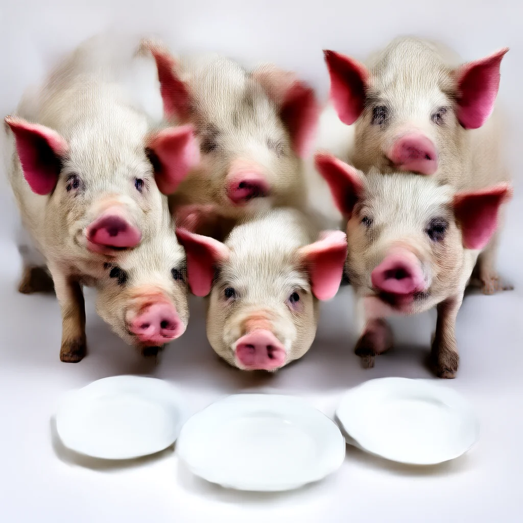 |
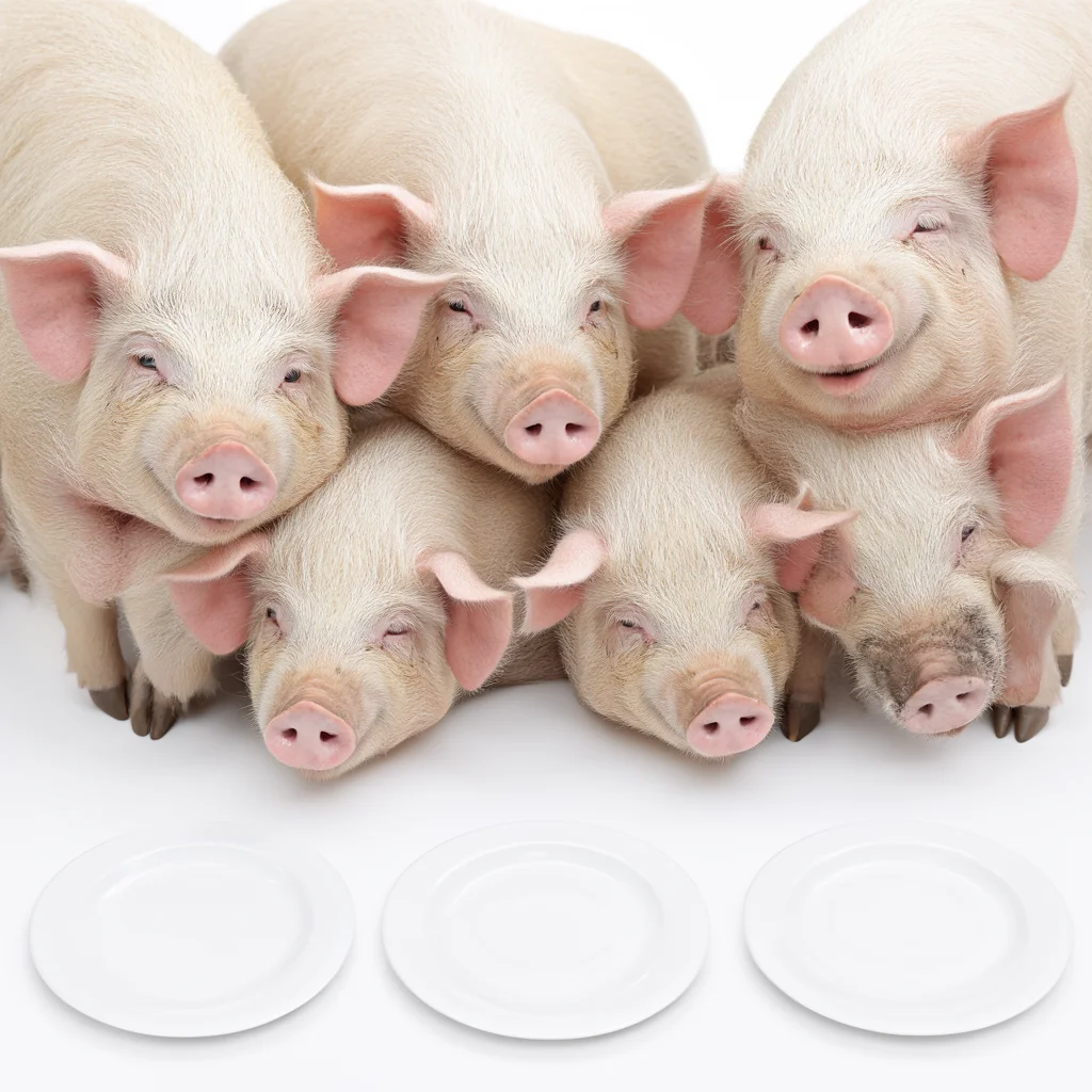 |
Worse: about seven pigs instead of four. |
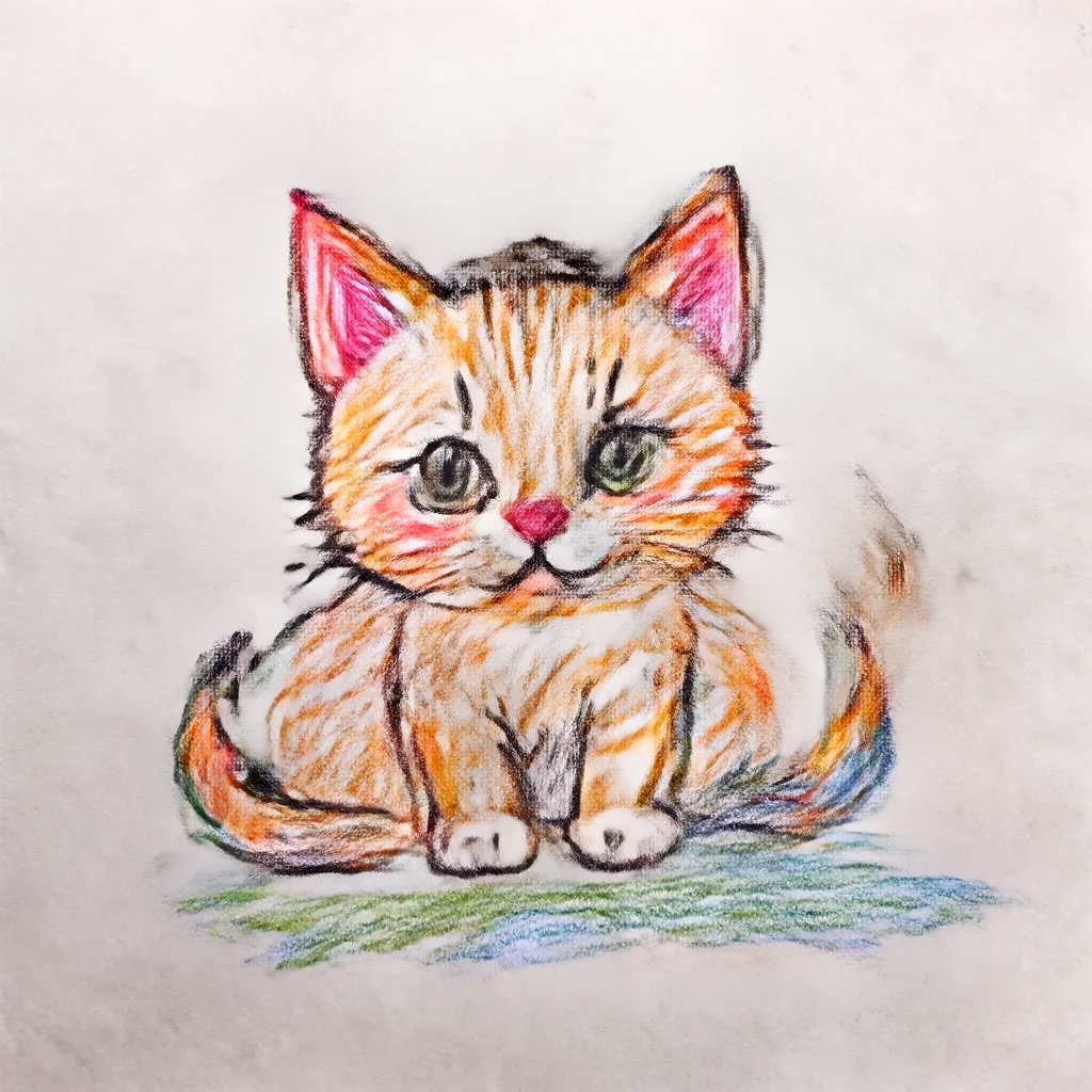
| a crayon doodle of a kitten | 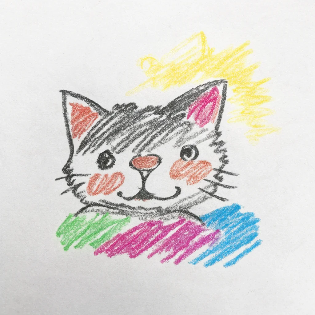 |
 |
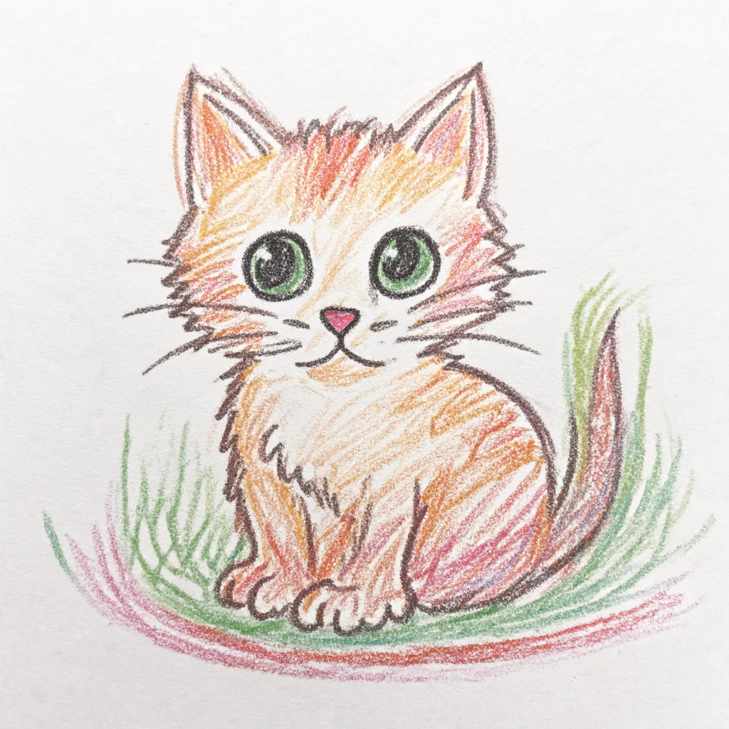 |
Style drifts from a child's doodle to a polished drawing. |
| hulk washing cinderella | 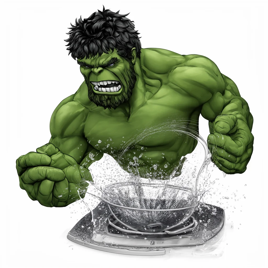 |
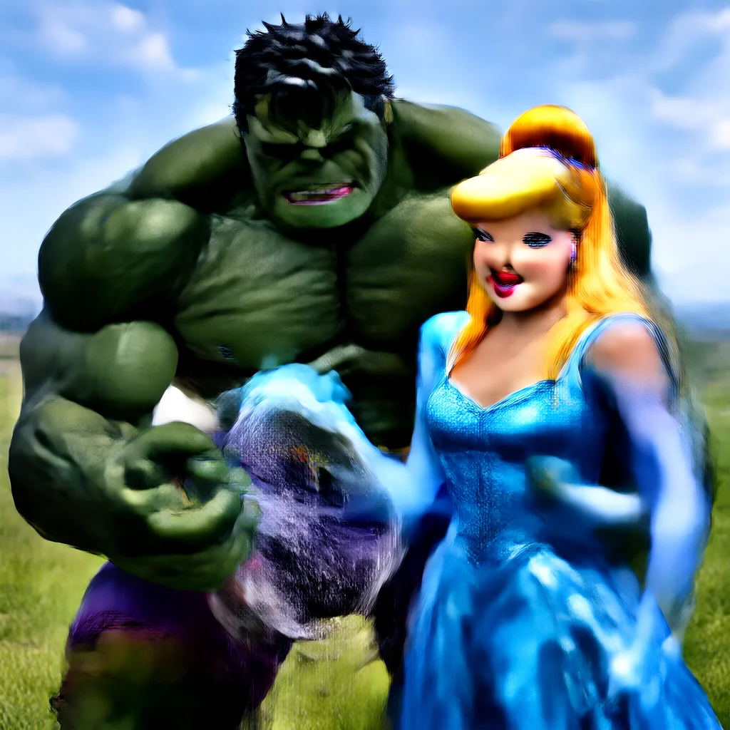 |
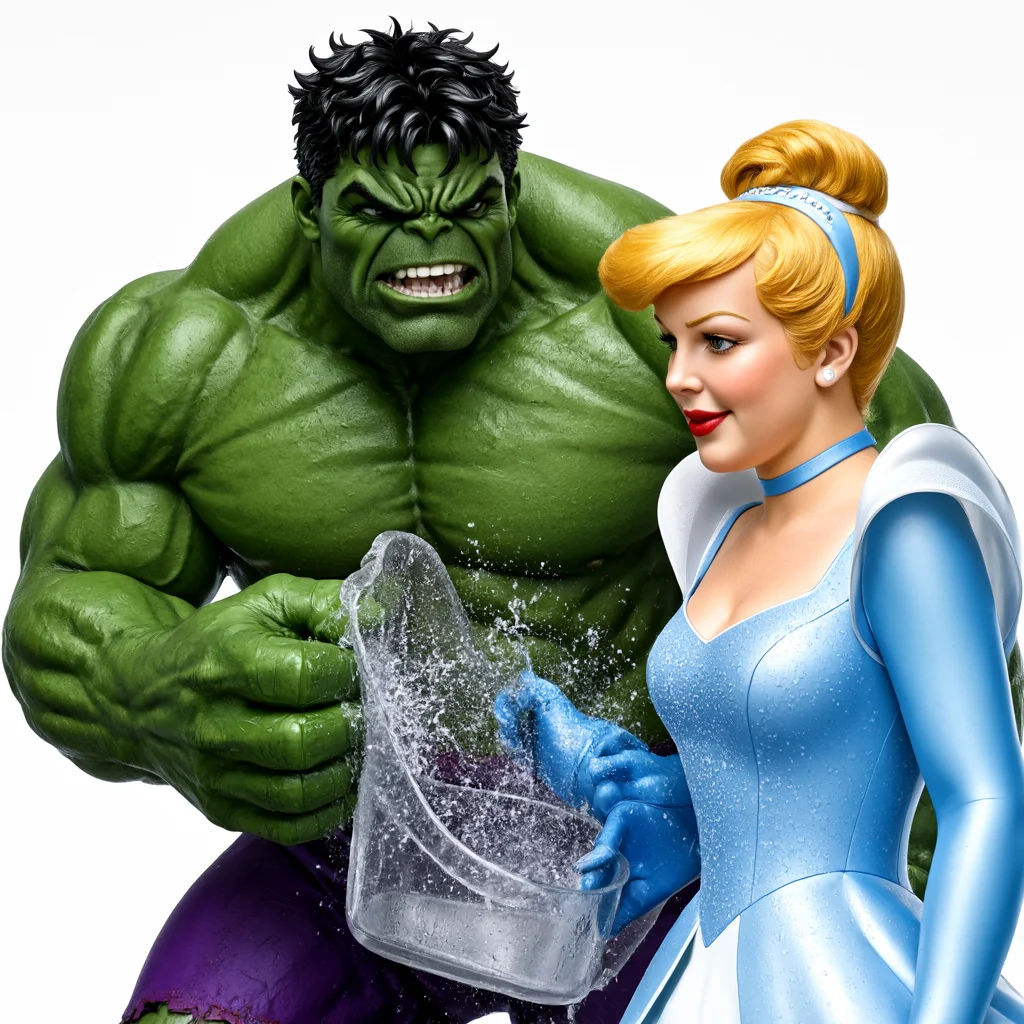 |
Better: Base drops Cinderella; ours draws both. |
| website, "AMOGUS" |  |
 |
 |
Better: Base makes a poster; ours lays out a web page. |
What broke the first attempt: numerics of the target
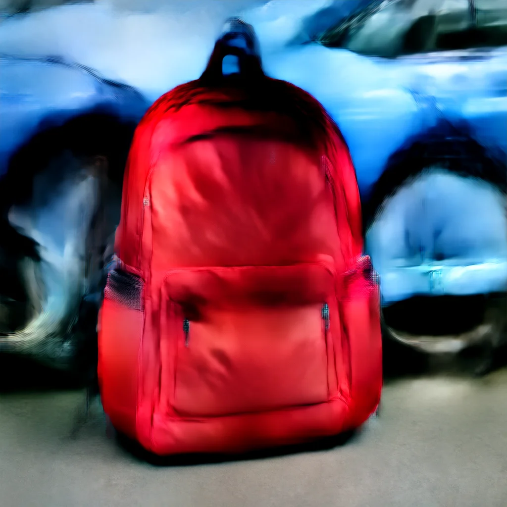
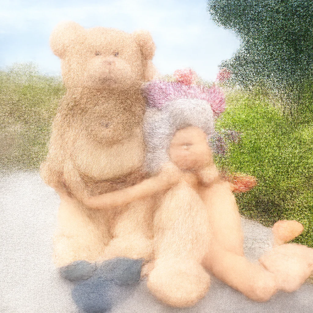
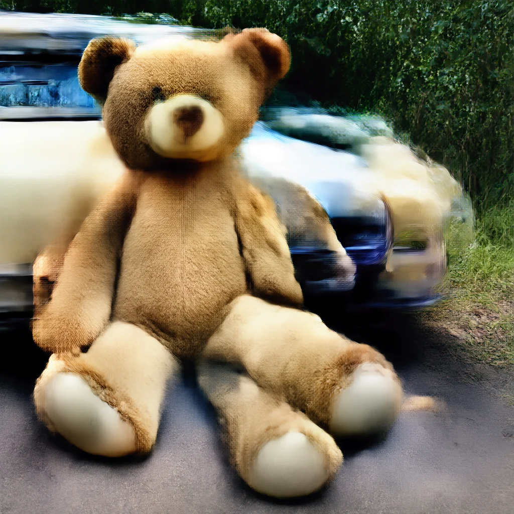
Our first full run (v1) produced shapeless blobs at 1–4 steps. Most of the damage came from the finite difference in .
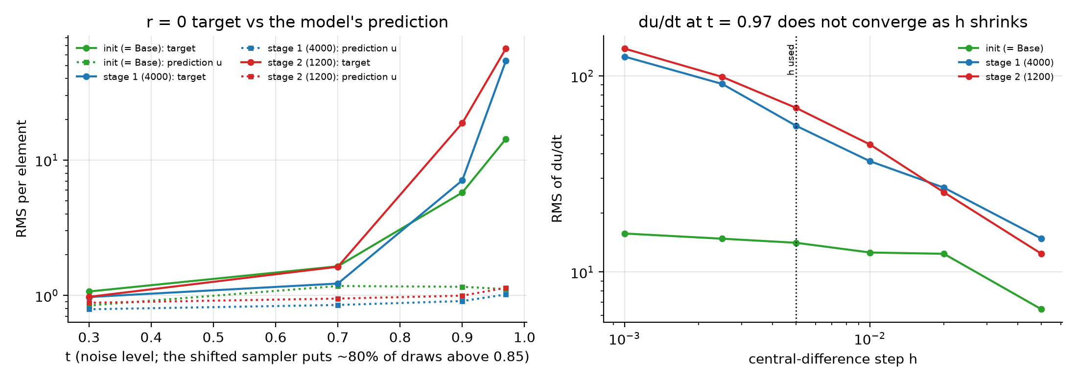
FLUX embeds time with sinusoids of . The fastest channel, , repeats every in . BFL's reference code stores timesteps in bf16, which keeps 8 significant bits: in the representable values are apart, so neighbouring bf16 times sit 3.9 radians apart in that channel (right panel below). v1 used . So often rounded to the same value, which silently drops the term, or to two neighbours 0.0039 apart, divided by . The two passes also ran in bf16 arithmetic, whose rounding noise gets amplified by .
We measured the target against a full-fp32 reference on the actual 5.5B model:
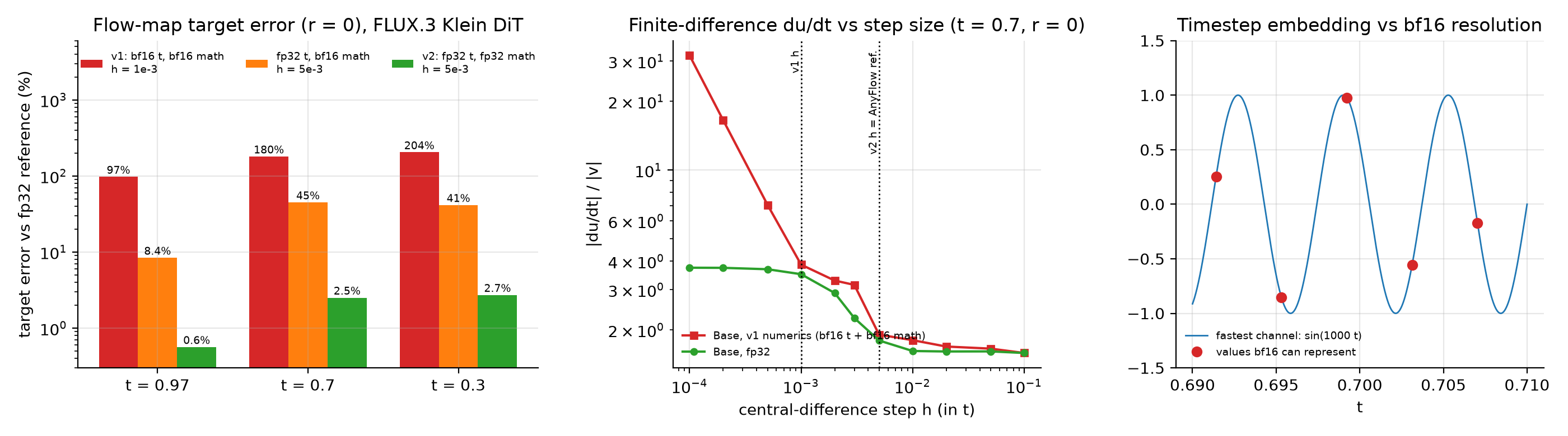
| Numerics | t = 0.97 | t = 0.7 | t = 0.3 |
|---|---|---|---|
| v1: bf16 timesteps, bf16 math, h = 0.001 | 97% | 180% | 204% |
| bf16 timesteps only (fp32 math), h = 0.001 | 58% | 106% | 9.5% |
| fp32 timesteps, bf16 math, h = 0.005 | 8.4% | 45% | 41% |
| v2: fp32 timesteps, fp32 math (TF32), h = 0.005 | 0.6% | 2.5% | 2.7% |
Rounding alone hurts less at because bf16 spacing there is 4× finer (0.00098). v2 keeps timesteps in fp32, runs the two difference passes with every linear layer upcast to fp32 (no fp32 copy of the weights needed), and uses AnyFlow's . We kept at the paper's value instead of shrinking it: at this scale the network's derivative itself depends on (in fp32, and give targets 21–74% apart), because of those fast embedding channels.
Three smaller bugs were fixed at the same time:
- v1 copied the time embedding into
ref_time_in. With additive conditioning, that doubled the time signal at initialisation. It is now zero-initialised. - The 50/25/25 split of time pairs was done per GPU with batch 1, and Python's
round(0.5) == 0silently removed the and anchors. It now runs over the global batch, rounding half up. - v1 did not apply FLUX's time shift during training.
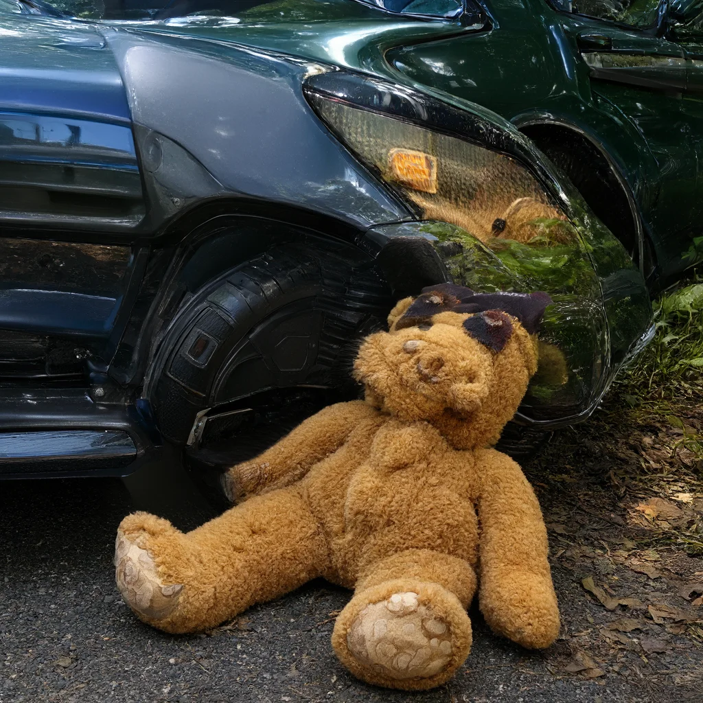
Same noise, Stage 1, v1 (with all four bugs, after 6,000 steps) vs v2 (after 4,000 steps):
| Prompt | v1, 1 step | v1, 4 steps | v2, 1 step | v2, 4 steps |
|---|---|---|---|---|
| a red backpack and a blue car | 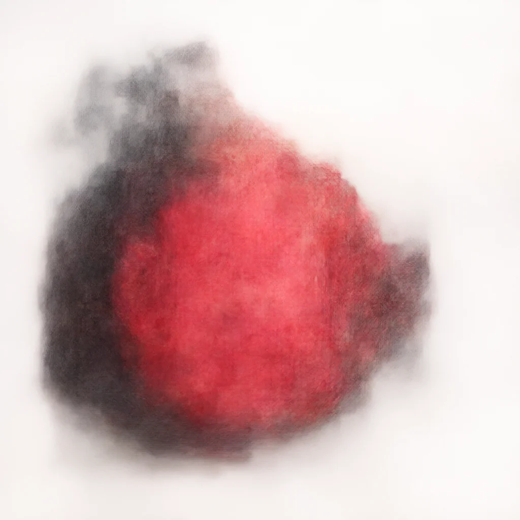 |
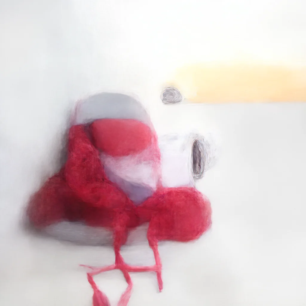 |
 |
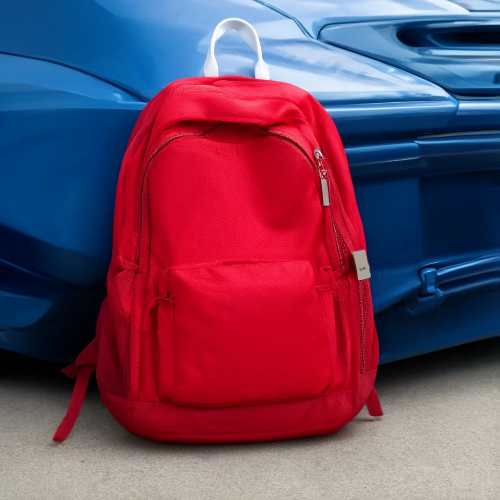 |
| photo, a teddy bear next to car … | 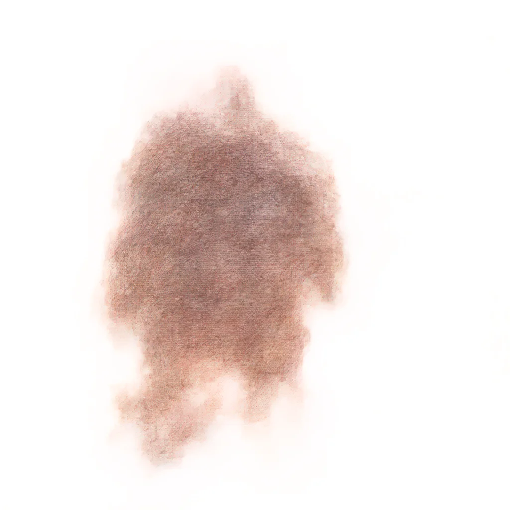 |
 |
 |
 |
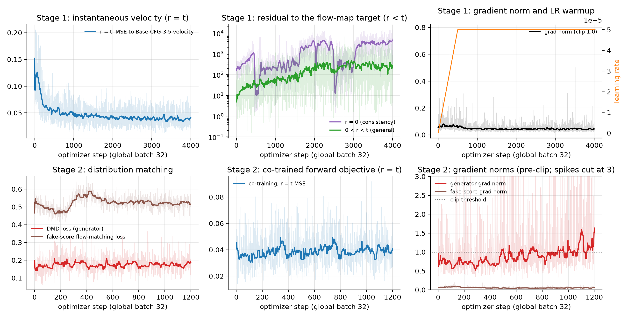
An open problem: the target at high noise. Even with clean numerics, the target can't be learned everywhere. At its RMS is 14 at initialisation, 54 after stage 1 and 67 after stage 2, while the model's output is about 1. The derivative term dominates, and it keeps growing as shrinks instead of converging. The trained network has developed fast wiggles in near pure noise, which Base doesn't have. The model doesn't fit these samples (the residual equals the target). The adaptive weight keeps them harmless by giving each one the loss scale of an average sample. That is why the stage-1 objective looks flat while the raw residual grows about 20× (training curves above). Stage 2 then repairs few-step quality directly from samples. A smoother time conditioning or an exact JVP derivative is the obvious next experiment.
Takeaways and limitations
- The recipe transfers. AnyFlow's two stages carry over from video to a 5.5B image model with just a LoRA and about a day on one node.
- Numerics are part of the method. A finite-difference target needs fp32 time and arithmetic, and its is a hyperparameter, not a precision knob.
- The two stages trade off differently. Stage 1 is an honest any-step model: it keeps Base's diversity and improves with more steps. Stage 2 buys few-step quality at the cost of some diversity and colour fidelity.
- Limitations. Automatic metrics only (no human study), 128 prompts, no comparison with BFL's 16-step distilled Klein, LoRA rather than full fine-tuning, and the high-noise target problem above.
References
- Black Forest Labs. FLUX 3 Image Klein: open weights, 5.6B parameters. Blog post, 2026.
- Y. Gu, G. Fang, Y. Jiang et al. AnyFlow: Any-Step Video Diffusion Model with On-Policy Flow Map Distillation. arXiv:2605.13724, 2026.
- Y. Lipman, R. T. Q. Chen, H. Ben-Hamu et al. Flow Matching for Generative Modeling. ICLR, 2023. X. Liu, C. Gong, Q. Liu. Flow Straight and Fast: Learning to Generate and Transfer Data with Rectified Flow. ICLR, 2023.
- N. M. Boffi, M. S. Albergo, E. Vanden-Eijnden. Flow Map Matching with Stochastic Interpolants: A Mathematical Framework for Consistency Models. arXiv:2406.07507, 2024. A. Sabour, S. Fidler, K. Kreis. Align Your Flow: Scaling Continuous-Time Flow Map Distillation. arXiv:2506.14603, 2025.
- Z. Geng, M. Deng, X. Bai et al. Mean Flows for One-step Generative Modeling. arXiv:2505.13447, 2025.
- Z. Wang, Y. Zhang, X. Yue et al. Transition Models: Rethinking the Generative Learning Objective. arXiv:2509.04394, 2025.
- T. Yin, M. Gharbi, R. Zhang et al. One-step Diffusion with Distribution Matching Distillation. CVPR, 2024. T. Yin, M. Gharbi, T. Park et al. Improved Distribution Matching Distillation for Fast Image Synthesis. NeurIPS, 2024.
- Metrics. PickScore: Y. Kirstain, A. Polyak, U. Singer et al. Pick-a-Pic: An Open Dataset of User Preferences for Text-to-Image Generation. NeurIPS, 2023. HPSv2: X. Wu, Y. Hao, K. Sun et al. Human Preference Score v2. arXiv:2306.09341, 2023. CLIP score: J. Hessel, A. Holtzman, M. Forbes et al. CLIPScore: A Reference-free Evaluation Metric for Image Captioning. EMNLP, 2021. LPIPS: R. Zhang, P. Isola, A. A. Efros et al. The Unreasonable Effectiveness of Deep Features as a Perceptual Metric. CVPR, 2018. DINOv2: M. Oquab, T. Darcet, T. Moutakanni et al. DINOv2: Learning Robust Visual Features without Supervision. TMLR, 2024.